Overview
This project is a “digital restoration” of Aneesur Rahman’s seminal 1964 paper, Correlations in the Motion of Atoms in Liquid Argon. While the physics of liquid argon is a solved problem, the challenge lies in bridging the gap between 1960s mainframe constraints and 2025 software architecture.
I replicated the simulation using LAMMPS and built a custom, production-grade Python analysis pipeline to process the trajectory data. The project demonstrates how modern tooling (uv, type hinting, vectorized NumPy) can transform academic “write-once” scripts into a robust, reproducible research toolkit.
Features
The Analysis Pipeline
I architected a modular Python package (argon_sim) designed for performance and maintainability.
- Intelligent Caching System: MD analysis is compute-intensive ($O(N^2)$). I implemented a decorator-based caching layer (
@cached_computation) that hashes source file modification times and function arguments. This ensures expensive calculations (like RDF or Van Hove correlations) are only re-run when the underlying trajectory or parameters actually change. - Vectorization & Optimization: To handle the $N^2$ complexity of pair-wise interactions without C++ extensions, I utilized NumPy broadcasting. For example, the Mean Square Displacement (MSD) calculation is fully vectorized, with a fallback “chunked” implementation to handle memory overflows on smaller machines.
- Modern Python Tooling:
- Dependency Management: Used
uvfor deterministic environment locking (sub-second resolution). - Type Safety: 100% type-hinted codebase for static analysis compliance.
- Automation: A robust
Makefileabstracts the complex workflow (simulation → analysis → figure generation) into single commands (e.g.,make figure-5).
- Dependency Management: Used
The Simulation Strategy
I used LAMMPS for the MD engine but strictly adhered to Rahman’s physical parameters while modernizing the stability mechanisms.
- Integration: Replaced Rahman’s predictor-corrector method with the modern standard Velocity Verlet algorithm (2 fs timestep).
- Equilibration: I implemented a 500 ps NVT equilibration phase to properly melt the FCC crystal structure before the NVE production run.
- Intellectual Honesty: The
in.argonscript explicitly documents every deviation from the original methodology (e.g., energy minimization) and the justification for ensuring numerical stability.
Usage
The project uses a Makefile to automate the workflow. Run make all to execute the LAMMPS simulation and generate all analysis figures.
Results
The replication achieved high quantitative agreement with the historical data, validating both the simulation parameters and the custom analysis code.
| Property | Rahman (1964) | This Work | Notes |
|---|---|---|---|
| Diffusion Coefficient ($D$) | $2.43 \x10^{-5}$ cm²/s | $2.47 \x10^{-5}$ cm²/s | Agreement within 2% |
| RDF First Peak | $3.7$ Å | $3.82$ Å | Slight shift |
| Velocity Dist. Width ($e^{-1/2}$) | $1.77$ | $1.77$ | Exact match to theoretical Maxwell-Boltzmann |
Visual Replication
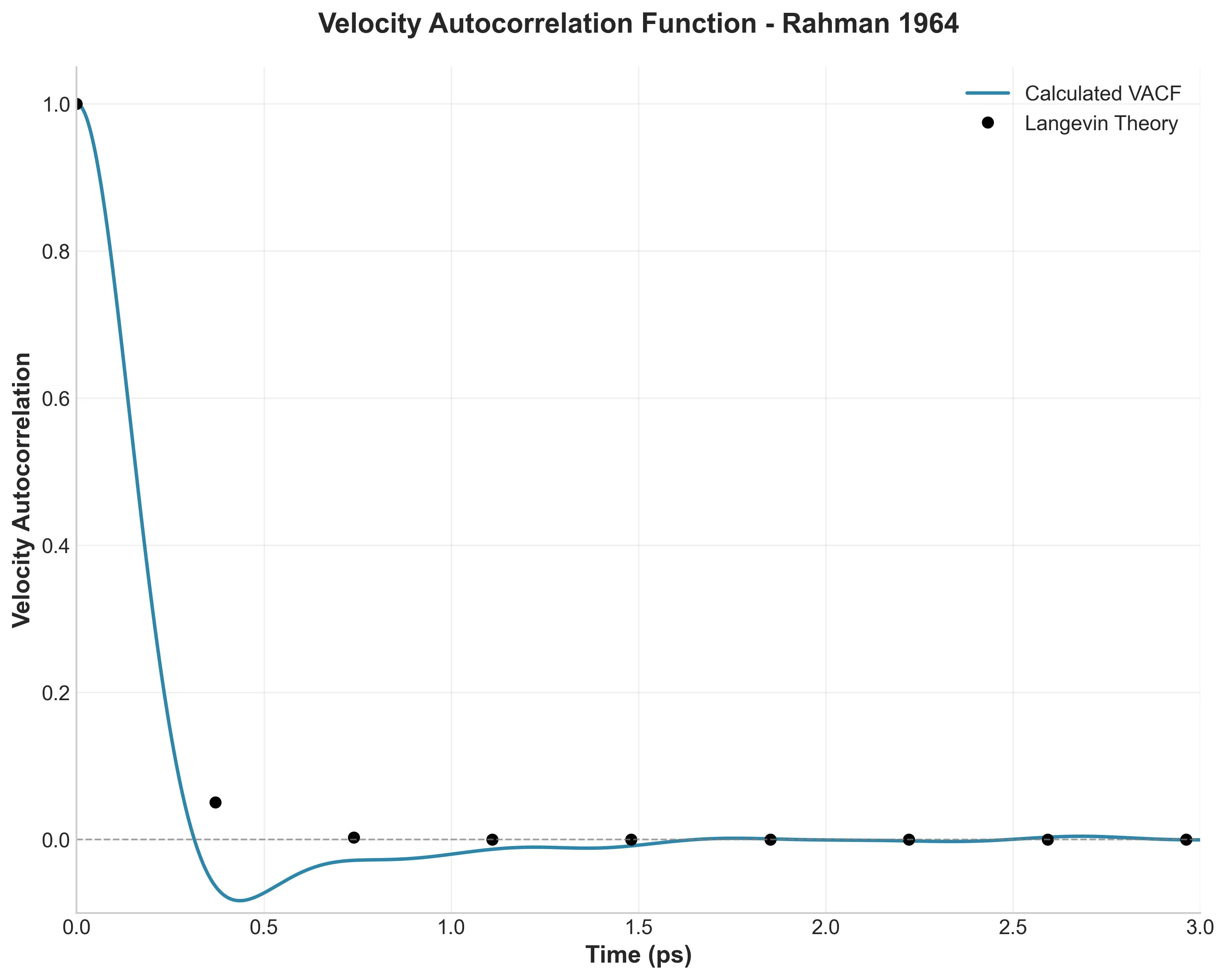
I used Matplotlib to digitally recreate Rahman’s hand-drawn plots, confirming signatures like the negative region in the Velocity Autocorrelation Function (VACF), which provided the first evidence of the “cage effect” in simple liquids.

Challenges & Learnings
- Unit Hell: Rahman’s paper uses a mix of reduced units and CGS. Mapping these to LAMMPS’s
realunits required a dedicatedconstants.pymodule and rigorous unit testing to prevent dimensional errors. - Fourier Transforms: Calculating the Structure Factor $S(k)$ from $g(r)$ required implementing a manual 3D Fourier transform for spherical symmetry, as standard FFT packages do not account for the radial shell integration implicit in liquid structure analysis.
- Code as a Liability: Early in the project, I realized that re-running analysis scripts was becoming a bottleneck. This drove the decision to build the caching infrastructure, reinforcing the lesson that investing in developer tooling pays off even in small-scale scientific projects.
Related Work
The full methodology and physics are documented in the companion blog post: