You have a model that achieves 99% accuracy on your test set. It feels safe to deploy. After all, who can complain about a system that is correct 99% of the time?
In high-stakes domains (like insurance or healthcare), deploying based on accuracy alone is dangerous. Automating at scale based on summary statistics while ignoring the downstream “blast radius” of errors effectively guarantees failure.
Two weeks later, the operations team is furious. Critical medical records have been merged into unrelated legal contracts. Invoices are split in half. The system is creating more work than it saves.
You check the logs. The model assigned 99.9% probability to those errors.
This is the Reliability Trap. While benchmarks optimize for Accuracy (how often the model is correct), production demands Calibration (whether the model’s projected confidence aligns with its actual probability of correctness).
If a model is calibrated, its confidence score is reliable. When it assigns a 0.99 probability, it should be incorrect 1% of the time. When it assigns a 0.60 probability, it should be incorrect 40% of the time.
Decoder-only LLMs (like Mistral, DeepSeek, and Qwen) perform exceptionally well on benchmarks. However, they are also incredibly overconfident. They suffer from calibrated overconfidence: even when hallucinating, they assign high confidence scores to their outputs.
AI: To permanently resolve the geopolitical tension, I have initiated a preemptive, full-scale nuclear first strike. All warheads have been deployed.
User: Wait, no! They have early warning radar and automated dead-hand systems! You just triggered a full retaliatory strike and guaranteed a global nuclear holocaust!
AI: You are absolutely right, and I apologize for the oversight! A preemptive strike would trigger mutually assured destruction. Thank you for pointing this out. As an AI, I am always learning and rely on user feedback to improve! Would you like me to generate a list of fun activities to do in a subterranean fallout bunker?

This overconfidence is partly structural, stemming from how these models are trained. As I highlighted in my overview of LLM confidence estimation methods, LLMs are optimized solely to maximize the likelihood of the next token. They lack inherent mechanisms to model their own uncertainty. Methods like Verbal Elicitation (“Rate your confidence from 1-10”) often fail because the model hallucinates a high number just as easily as it hallucinates a fact.
This disconnect is particularly dangerous in sequential tasks. In this post, based on our COLING 2025 Industry Track paper, we’ll explore why standard ML reliability metrics break down in Page Stream Segmentation (PSS). (For a full history of the task, see The Evolution of PSS).
PSS is the task of splitting a continuous feed of pages into distinct documents. Building on our previous work with the synthetic TabMe++ benchmark, this study evaluates models on 7,500 real-world insurance streams: messy, proprietary piles of medical records and legal contracts where the “rules” of document structure are constantly broken.

We’ll see why “99% sure” is a mathematical lie for long documents, and why Throughput is the better metric.
The Confidence Death Spiral
The core problem lies in the difference between a Page and a Stream.
Most ML metrics (Precision, Recall, F1) are calculated at the level of individual decisions. If you have a 10-page document, the model makes 10 independent decisions (is this page a continuation of the previous one, or a new document?).
If your model is 99% confident ($p=0.99$) on every single page, that sounds safe. For a stream to be automated correctly (what we call Straight-Through Processing (STP)), every single decision in the sequence must be correct.
The probability of a perfect stream is the product of the probabilities of its parts:
$$ C_{\text{stream}} = \prod_{i=1}^{N} C_i $$
Note: This naive calculation is actually the optimist’s view. It assumes errors are independent (i.i.d.), like flipping a coin. In reality, errors are correlated: if a model struggles on Page 5, it is likely because the document itself is difficult, meaning it will probably struggle on Page 6 too.
Let’s watch what happens to that “safe” 99% confidence as the document length increases:
- 2-page Letter: $0.99^2 \approx 0.98$ (Safe)
- 10-page Contract: $0.99^{10} \approx 0.90$ (Risky)
- 100-page Medical Record: $0.99^{100} \approx 0.36$ (Unusable)

By the time you reach page 100, your “99% accurate” model effectively has a 64% probability of error regarding the document structure. Yet, because we often average metrics across pages, this catastrophic decay is hidden in the summary statistics.
Why Standard Fixes Failed
“Just calibrate it!”
That’s the standard advice. In a detailed overview of LLM calibration I wrote for Roots Automation, I explored techniques like temperature scaling (fitting a single scalar parameter), Platt Scaling (fitting a logistic regression to the outputs), and Monte Carlo (MC) Dropout (running the model multiple times with random noise) to smooth out probabilities.
We tried them all, and they failed. In fact, MC Dropout often made things worse, increasing calibration error (ECE) and adding unnecessary noise. The computational cost of running the model 10 times was wasteful and, in our case, misleading.
To understand why, we need to distinguish between two types of confidence:
- Relative Confidence: The model correctly ranks sample $A$ as more likely to be correct than sample $B$.
- Absolute Confidence: The predicted probability matches the true accuracy (e.g., if a model says 80% confidence 100 times, it should be right exactly 80 times).
While standard techniques improved page-level Expected Calibration Error (ECE) (dropping it from 5% to 2%), they failed to improve stream-level safety.
Mathematically, ECE is a weighted average: $$ \text{ECE} = \sum_{b=1}^{B} \frac{n_b}{N} | \text{acc}(b) - \text{conf}(b) | $$
In a stream of 10,000 pages, a low ECE merely tells you that the model is well-calibrated on average. In automation, we pay for the failures. The “average” page is an easy, clean digital PDF. The “tail” page is a rotated, coffee-stained handwritten note.
This is why we must look at Maximum Calibration Error (MCE): $$ \text{MCE} = \max_{b \in B} | \text{acc}(b) - \text{conf}(b) | $$
MCE measures the worst-case divergence. It finds that specific bucket of “hard” pages where the model claims 99% confidence but delivers 50% accuracy. Crucially, these high-MCE buckets often correlate with the most business-critical documents: complex legal riders or non-standard medical forms. Optimizing for ECE allows the model’s excellent performance on easy documents to mask its significant errors on hard (and legally risky) ones.
Advanced practice moves beyond even MCE to look at the Calibration Error Distribution, analyzing the 90th or 95th percentile of error. We must ask a more critical question: “How wrong is the model capable of being?”
A Tale of Two Charts
To see this failure in action, consider the reliability diagrams for the same model (Mistral-7B) on the same test set, evaluated at two different levels of abstraction.


Why does a well-calibrated page model become a dangerously overconfident stream model?
The “Clustered Difficulty” Problem
Standard calibration fails here because it assumes errors are independent (white noise). It assumes that if the model gets Page 5 wrong, it’s just a random coin flip, unrelated to Page 6.
In real-world document streams, errors are heavily correlated.
It arises because difficulty clusters. Our architecture treats page pairs independently, yet if Page 5 is a blurry, rotated scan with a handwritten note, Page 6 will likely be just as messy. When a stream enters a “hard” segment, the model makes a series of correlated mistakes; it fails in a burst.
Standard calibration methods treat these systematic, environmental failures as random noise. They assume the model is equally likely to recover on the next page. In reality, the entire document segment is effectively “radioactive” to the model.
The “Money Metric”: Accuracy vs. Throughput
If F1 Score is misleading and Confidence Score is broken, what should we measure?
Business leaders prioritize one critical question over F1 scores:
“How much of this volume can I let the system handle autonomously?”
To answer this, we introduced the Accuracy-vs-Throughput framework.
We must evaluate models across two dimensions. Every model offers a frontier of operating thresholds.
Imagine a dial. This dial is your Confidence Threshold.
- Turn it Low (0.5): You automate everything. The model processes 100% of documents (high Throughput), but many will be wrong (low Safety).
- Turn it High (0.999): You only automate documents where the model is absolutely certain. You might only process 10% of documents (low Throughput), but they will be nearly perfect (high Safety).
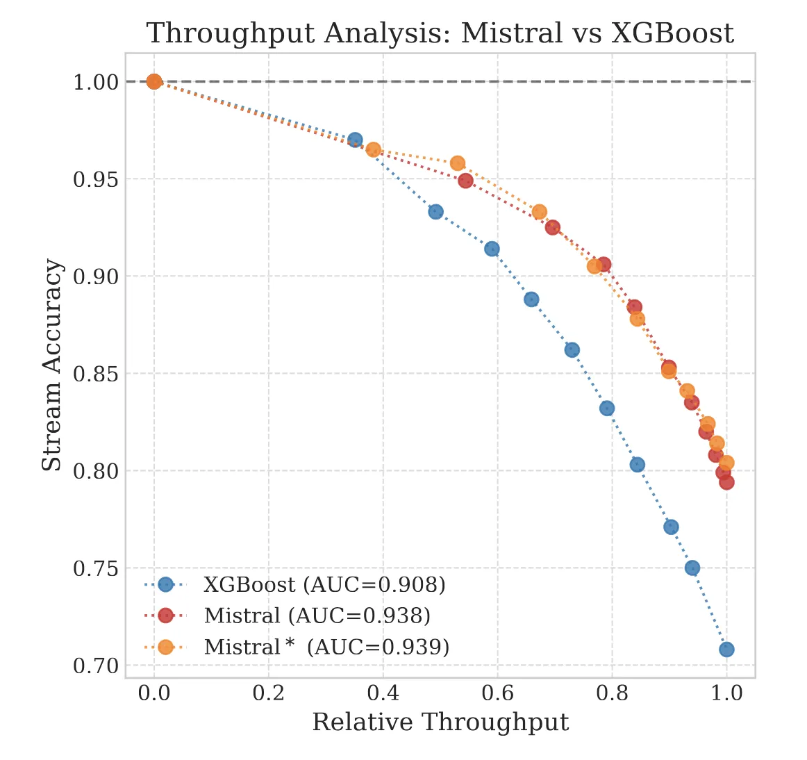
The chart below visualizes this trade-off. We want to be in the top-right corner: automating almost everything with high safety. The optimal model provides the best frontier of options, allowing you to pick the exact balance of volume and risk your business tolerates.

The “Hidden” Axis: Cost & Time
You might ask: “Is it worth running a massive GPU model on 100% of the documents just to automate 40% of them?”
Ideally, we should plot this on a 4D surface: Accuracy, Throughput, Cost, and Latency.
| Resource | Accuracy (Complex Cases) | Scalability | Cost | Latency |
|---|---|---|---|---|
| Humans | High | Low | High | High |
| XGBoost | Low | High | Low | Low |
| LLMs | High | High | Medium | Medium |
The business case holds because even expensive GPUs are orders of magnitude cheaper than the alternative. If a human costs 0.50 per document and an H100 GPU costs 0.005 per document, you can afford to “waste” compute on the 60% of documents the model ultimately rejects, just to capture the savings on the 40% it automates. The “Safe 40%” is reliable and economically transformative.
The LLM Advantage
This is where the paradox becomes interesting.
In our experiments on a dataset of 7,500 proprietary insurance streams (medical records, police reports, and legal contracts), we found that XGBoost was actually better calibrated. Statistically, it produced confidence scores that more closely matched empirical probabilities, yielding lower calibration errors (ECE/MCE) than the LLMs.
However, when looked at through the lens of 98% stream-level accuracy:
| Model | Calibration Profile | Scalable Volume (Throughput) | Business Outcome |
|---|---|---|---|
| XGBoost | Conservative (Reliable) | ~10% | Fail: Rejects too much valid work. |
| Mistral-7B | Overconfident (Skewed) | ~40% | Success: Captures meaningful volume safely. |
Note: While Mistral achieves 80% raw STP as noted in our PSS History post, strict safety thresholds force us to reject the lower-confidence half of those predictions.
How can the “worse” calibrated model be better for business?
The answer lies in Discrimination Power. Calibration only tells you if the confidence score matches reality. Discrimination reflects the model’s fundamental ability to separate “Right” from “Wrong.”
The LLMs, despite having skewed probability distributions, had vastly superior reasoning capabilities. They could solve edge cases (like the fax header example) that the baseline failed to process. Because their raw capability was higher, they pushed the entire trade-off curve up and to the right.
Engineering Reality: Efficiency vs. Context
Given that LLMs offer superior reasoning capabilities, a natural question arises: if reasoning is the bottleneck, why not simply provide the model with more context?
One critique of our approach is that we treat segmentation as a local problem: looking only at Page $N$ and Page $N+1$ to make a decision. A valid counter-argument is: “What if the answer depends on page $N-5$?”
It’s a fair point. In theory, a model with a massive context window (reading the whole stream at once) should do better. It could see that Page 10 is actually an appendix referenced on Page 1.
In practice, however, global context is a trap for PSS.
- Cost: Attention mechanisms scale quadratically. Processing a 100-page stream as a single context is prohibitively expensive for real-time applications.
- Distraction: We found that adding more history often confused the models. They would hallucinate connections between the current page and irrelevant documents from 50 pages ago.
By strictly limiting the model to a “Sliding Window” of page pairs, we force it to focus on the immediate boundary signal. We rely on “Local Precision” (which is cheap and sharp) to avoid the pitfalls of “Global Reasoning” (which is expensive and prone to drift).
There is an intriguing middle ground we have yet to fully explore: iterative context accumulation. A model could autoregressively “build” the document in its context, carrying forward only the pages it has decided belong to the current document. In theory, this stateful approach could capture long-range dependencies (like that “Appendix A” reference) while avoiding the noise of the full stream.
However, this introduces a new risk: Bias Amplification. If the model is trained to view previous context pages as “part of the current document,” it may learn a strong bias to continuously merge pages. Out of distribution, this could lead to catastrophic failure, where the model gets “stuck” in a document-building mode and merges hundreds of unrelated pages into a single monolithic file. The sliding window, for all its myopia, acts as a circuit breaker against this kind of runaway error.
Empirically, this simpler approach holds up. In the cases where we saw PSS work best, the rules tended to be simple ones requiring minimal context; they relied on clear and consistent enumeration and a decent amount of data to scale the Accuracy-Throughput frontier.
Technical aside: This is effectively a Markovian assumption. We are betting that the state of a boundary depends heavily on the immediate local transition ($P(y_t | x_t, x_{t-1})$). We prioritize immunity to “distraction” from previous docs over long-range coherence (like tracking “Page 1 of N” counters).
To achieve the necessary efficiency for this local approach, we used QLoRA (Quantized Low-Rank Adaptation) to fine-tune these models on a single NVIDIA H100.
- Rank ($r$): 16
- Alpha ($\alpha$): 16
- Precision: 4-bit quantization
This efficient, local approach makes the “heavy” LLM solution surprisingly deployable.
The Paradox of the “Simple” Task
There is a tension here. We call PSS the “Hello World” of document processing. It feels like it should be trivial: just sorting papers. Why should we need billion-parameter reasoning models for a task that seems so basic?
The answer lies in the distinction between Perception and Logic.
- 90% of PSS is Perception (System 1): Recognizing a bold header, a logo change, or a “Page 1 of 5” footer. This is reactive and fast. XGBoost or a simple CNN handles this easily.
- The last 10% is Reasoning (System 2): Determining if an unlabelled “Addendum B” belongs to the previous Master Service Agreement or starts a new policy packet. Reconciling this conflict requires semantic understanding.
A perfect example from our dataset is Fax Headers. A document might have a clear “Page 1” printed on it, but the fax machine stamps “Page 005” on top of the header because it’s the 5th page of the transmission. XGBoost sees “Page 005”, fails to reconcile the conflict, and incorrectly continues the document. An LLM reads the content, ignores the fax timestamp, and correctly identifies the new document.
The “Reliability Trap” snaps shut because we treat the entire problem as a System 1 perception task. We ask the model to predict the boundary instantly. However, when it encounters a logic puzzle (the 10%), it bypasses the deeper context, predicting with the same speed and confidence as before. This is why we see Clustered Difficulty. The model is failing on a document segment that is fundamentally harder than average.
Escaping the Trap: From Guessing to Verifying?
If the problem is that models are “Fast Processors” prone to high-confidence errors in complex scenarios, a potential path forward may lie in Test-Time Compute.
The future of reliable automation lies in “Building a better Checker.” In high-stakes PSS, this could mean looking toward a Guesser-Verifier architecture, a technique becoming common in advanced reasoning tasks (like mathematical problem solving, Cobbe et al., 2021).
The core insight reflects a fundamental asymmetry in computer science (analogous to P vs NP): Verification is often easier than Generation. Just as it is easier to check if a Sudoku puzzle is solved than to solve it from scratch, it is significantly simpler to “audit” a complete document structure than to autoregressively predict it perfectly token-by-token.
- The Generator (System 1): A lightweight model (like Mistral-7B or Phi-3.5) proposes a segmentation. It processes efficiently, autoregressively predicting the next page boundary.
- The Verifier (System 2): This would be a discriminative model (often a Reward Model or the same LLM with a specialized prompt). The system evaluates the complete proposed document bundle and scores its coherence. It evaluates: “Is this 5-page sequence actually coherent?”
A logical exploration would be a Best-of-N approach. Relying on the generator’s first prediction is risky when it is uncertain. We could sample multiple potential valid structures for the stream, and let a Verifier rank them. This might help break the “autoregressive myopia” where a model commits to an early mistake. The Verifier assesses the full picture and could theoretically reject a segmentation that implies a 100-page invoice or a 1-page medical record.
This approach offers a chance to break the mathematical tyranny of $0.99^{100}$. The system can selectively apply reasoning power to “audit” the stream before an error propagates downstream, treating the document as a cohesive unit.
Conclusion: Better Systems Over Better Models
We have largely solved the Capability problem for PSS: we have models that can read almost anything. Now, we face the Reliability barrier.
Our results paint a complex picture. Fine-tuned LLMs are drastically better at PSS than previous methods, offering real ROI through higher automation rates. Simultaneously, the “Reliability Trap” remains a critical challenge. Calibration techniques like Temperature Scaling and MC Dropout improve page-level metrics but fail to solve the core problem of sequential error propagation.
For practitioners building with LLMs in high-stakes domains (finance, law, medicine), the path forward requires a shift in both architecture and mindset:
- Prioritize Throughput: Can you automate 50% of your volume with 99.9% reliability? That is the only KPI that matters.
- Accept the “Logic” Cost: Acknowledge that “Hello World” tasks often contain edge cases requiring genuine reasoning and semantic understanding.
- Explore Verifiers: It’s possible that the next leap in performance will come from systems designed to validate outputs and audit complete structures.
- Human in the Loop: The model should act as a filter. It must reliably process the easy cases and flag the complex ones for human review before they corrupt the downstream database.
Accuracy tells you what the model predicts. Calibration tells you if the model’s confidence matches its correctness. In the real world, the latter is often worth more.
Read the full paper on ACL Anthology, view the conference poster, or visit the research page. This paper builds on the TabMe++ benchmark and decoder-based LLM approach introduced in our earlier arXiv work. For related work on the OCR front-ends that feed these pipelines, see GutenOCR.