Some papers invent entire fields. Aneesur Rahman’s 1964 paper, “Correlations in the Motion of Atoms in Liquid Argon”, is the “Hello World” of molecular dynamics (MD). Using a computer with less memory than a modern microwave, Rahman solved Newton’s equations for 864 atoms and proved that liquids have distinct, quantifiable structure.
The physics of liquid argon is a solved problem. We know the answer.
So, why replicate it in 2025? To apply modern engineering standards to legacy science.
This project served as an exercise in software archaeology: taking a vintage scientific workflow and rebuilding it with a production-grade Python analysis pipeline. I wanted to see if I could replace Rahman’s “write-once” Fortran mentality with modern reproducibility, type safety, and intelligent caching.
The full source code is available on GitHub. The complete project overview, including analysis results and pipeline architecture, is on the Rahman 1964 Replication project page.
Engineering the Pipeline
The most interesting part of this project isn’t the simulation engine (LAMMPS handles that); it’s the architecture of the analysis suite. MD analysis is computationally expensive ($O(N^2)$), and iterating on plots can be painfully slow if you re-compute trajectory data every time.
Why bother? Don’t modern MD packages come with analysis tools? Well, some say that writing is thinking. Sometimes getting into the weeds of how an algorithm works or an analysis is performed, you gain insights and a deeper understanding that might be obscured by a plug-and-play tool.
Intelligent Caching
I architected the argon_sim package with a decorator-based caching layer. The system hashes the source file’s modification time and the function’s arguments to avoid re-calculating the Radial Distribution Function (RDF) or Van Hove correlations on every script run.
@cached_computation("gr")
def compute_radial_distribution(filename: str, dr: float = 0.05):
    # ... expensive O(N^2) distance calculations ...
    return r_values, g_r, density
If I tweak a plot axis, the script runs instantly, loading pre-computed arrays from disk. If I change the simulation trajectory, the cache invalidates automatically. This reduced my feedback loop from minutes to milliseconds.
Vectorization & Memory Management
Rahman likely relied on nested loops. Python is too slow for that. I utilized NumPy broadcasting to vectorize the calculation of atomic displacements.
However, calculating an $864 \x864$ distance matrix for 5,000 frames consumes significant RAM. I implemented a chunked MSD (Mean Square Displacement) algorithm that processes the trajectory in blocks, balancing vectorization speed with memory constraints. This allows the analysis to scale from Rahman’s 864 atoms to millions without crashing a laptop.
Reproducibility as a Feature
Academic code is notorious for “it works on my machine.” To combat this, I used uv for dependency management, locking the exact environment state. The entire workflow (from simulation to final figure generation) is abstracted into a Makefile.
# One command to run the physics, analyze data, and generate plots
make workflow
The Simulation: 1964 vs. 2025
I preserved Rahman’s physical parameters exactly to ensure a fair comparison:
- System: 864 Argon atoms
- Potential: Lennard-Jones ($\sigma = 3.4$ Å, $\epsilon/k_B = 120$ K)
- Target: 94.4 K, 1.374 g/cm³
However, I modernized the numerical methods to ensure stability:
| Feature | Rahman (1964) | This Work (2025) | Why it Matters |
|---|---|---|---|
| Integration | Predictor-Corrector | Velocity Verlet | Better energy conservation over long runs |
| Timestep | 10 fs | 2 fs | Rahman’s step was aggressive; 2 fs ensures numerical stability |
| Equilibration | Velocity Scaling | 500ps NVT | Rahman couldn’t afford long equilibrations; I melted the crystal properly to remove bias |
The production run lasted 10 ps in the NVE ensemble, generating 5,001 frames. Temperature remained within 1% of target with an RMS fluctuation of just 0.0165, substantially more stable than Rahman could achieve with 1960s hardware.
Validation Results
The replication was quantitatively successful. The analysis pipeline faithfully reproduced every key signature of liquid argon.
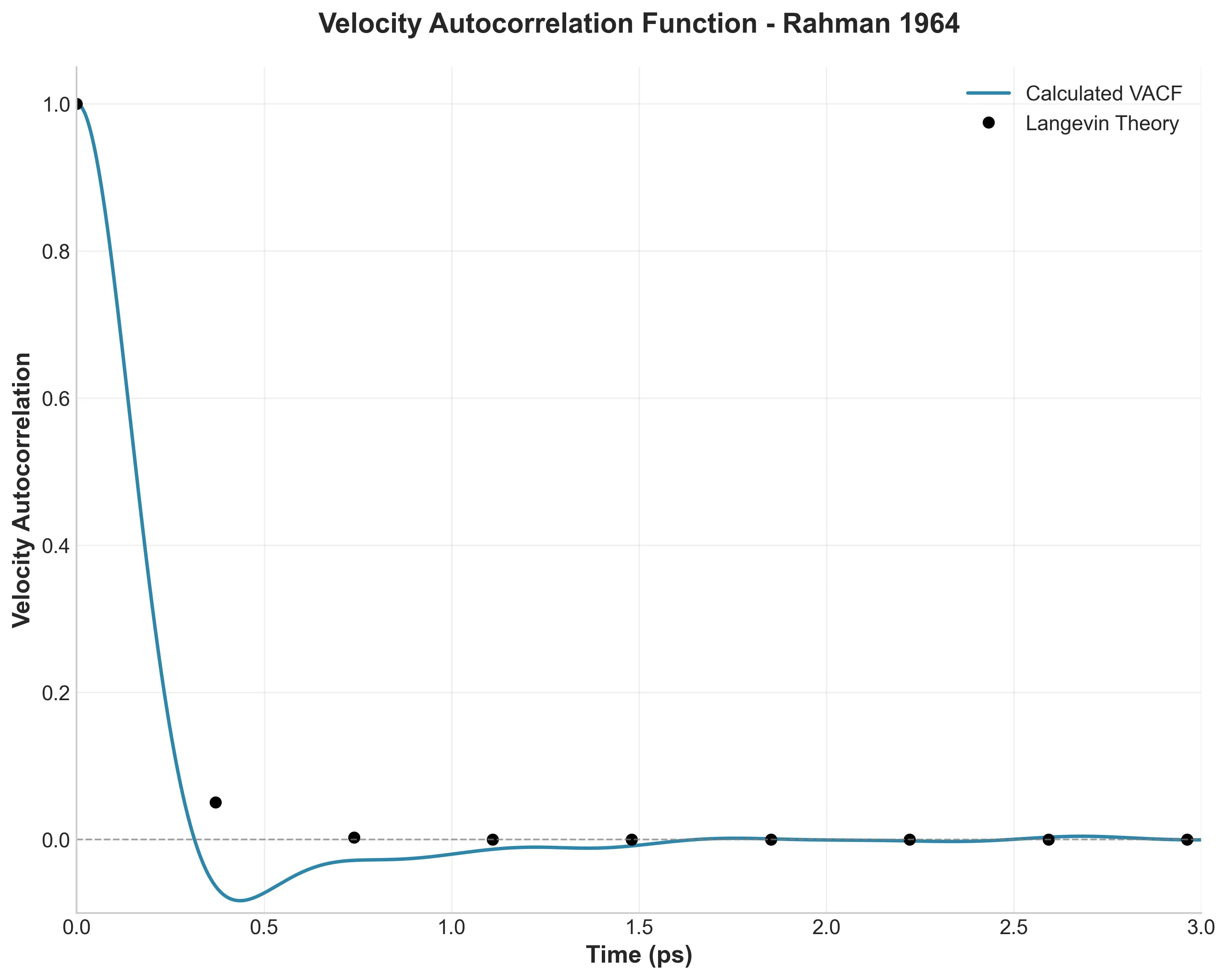
The Cage Effect
This is the paper’s crown jewel. In a gas, velocity correlations decay exponentially. In a liquid, Rahman discovered that atoms get trapped by their neighbors and bounce back, causing the correlation to go negative.

My simulation captures this minimum at -0.083, matching Rahman’s observation. The Fourier transform of this data (the frequency spectrum) reveals a peak at $\beta \approx 0.25$, physically representing the frequency of atomic collisions within the cage.

Structural Fingerprints
The Radial Distribution Function $g(r)$ and its Fourier transform, the Structure Factor $S(k)$, are the “fingerprints” of a liquid’s structure.

The agreement here is striking. My first peak appeared at 3.82 Å (Rahman: 3.7 Å). The slight discrepancy is likely due to my improved equilibration method, which allowed the system to relax into a more natural liquid state than Rahman’s 1960s hardware allowed.
Diffusion and Non-Gaussian Behavior
By calculating the Mean Square Displacement (MSD), I derived a diffusion coefficient of $D = 2.47 \x10^{-5}$ cm²/s, which deviates only 2% from Rahman’s reported $2.43 \x10^{-5}$.

More interestingly, I reproduced the “Non-Gaussian” parameters. Standard diffusion assumes a Gaussian distribution of displacements. Rahman found (and I confirmed) that liquid atoms deviate from this. They exhibit “jump” and “wait” dynamics, a behavior that standard Brownian motion models fail to capture.

Advanced Analysis: Van Hove Functions
Rahman also explored advanced properties like the Van Hove correlation function $G(r,t)$, which describes how liquid structure evolves over time.
 at two time points")
At 1.0 ps, the structure remains well-defined with clear shells. By 2.5 ps, it becomes increasingly diffuse. Rahman compared this evolution to theoretical predictions (the Vineyard approximation) and found that theory predicted overly rapid structural decay. My results confirm this finding.

System Validation
Before analyzing physics, basic sanity checks confirmed proper thermal equilibrium.

Mean temperature was 94.73 K (just 0.33 K off target) with a standard deviation of 1.56 K. That’s significantly better stability than Rahman achieved with 1960s computational resources.

The velocity distribution from 12.9 million velocity components produces a perfect Maxwell-Boltzmann distribution, as expected for thermal equilibrium. The distribution widths at various heights match Rahman’s results remarkably well: 1.77, 2.48, and 3.56 compared to his 1.77, 2.52, and 3.52.
Conclusion
Replicating a 60-year-old paper might seem like a solved puzzle, but it teaches a valuable lesson in computational science. Rahman relied on brilliance and raw mathematical intuition because he lacked compute power. Today, pairing our massive compute power with strict software rigor unlocks even greater reliability.
Applying modern software engineering (modular architecture, caching, and automated workflows) to classical physics reproduces the past and builds a foundation that makes the next discovery easier, faster, and more reliable.
The quantitative agreement is striking: diffusion coefficients within 2%, structural peaks within 0.1 Å, velocity distributions matching to three significant figures. This level of reproducibility, achieved with completely different hardware and software, validates something fundamental: Rahman’s physical model was remarkably sound, and his computational methodology was scientifically rigorous despite 1960s constraints.
The cage effect, velocity correlations, and structural evolution are fundamental characteristics of how matter behaves at the atomic scale, as relevant today as they were six decades ago.