Implementing the Müller-Brown Potential in PyTorch

Introduction

The Müller-Brown potential is one of computational chemistry’s most enduring test cases—a simple two-dimensional surface that has challenged algorithms for nearly five decades.

In the 1970s, researchers faced a fundamental problem: how do you test algorithms for finding transition states on molecular potential energy surfaces? Quantum chemistry calculations were expensive, making algorithm development slow and costly. Klaus Müller and L.D. Brown’s 1979 solution¹ was elegant: create a simple analytical function that captures the essential challenges of real chemical systems.

The Müller-Brown potential succeeds because it balances simplicity with complexity. Using just two coordinates and a handful of parameters, it creates multiple minima, saddle points, and curved reaction pathways. It’s complex enough to break naive algorithms but simple enough to provide known ground truth.

This post shows how to implement this classic potential in PyTorch, comparing analytical derivatives with automatic differentiation and demonstrating its continued relevance for modern computational chemistry.

The Problem: Finding Saddle Points in the 1970s

In the 1970s, finding energy minima was straightforward—follow the gradient downhill. But finding transition states was much harder. These saddle points are maxima along the reaction coordinate but minima in all other directions, like being at the top of a mountain pass.

Standard optimization algorithms go downhill by design. Point them at a saddle point, and they slide into the nearest valley. Specialized algorithms were needed to navigate this mixed landscape of ups and downs.

The computational reality made this worse. Early quantum chemistry programs like ATMOL and Gaussian made energy calculations possible, but each computation was expensive. Gradients required even more resources, and second derivatives were rarely computed.

This created a catch-22: sophisticated algorithms were needed to find saddle points, but researchers couldn’t afford to test them on real molecular systems. Every calculation was a major investment of time and resources.

Müller and Brown’s Solution

Müller and Brown’s insight was to create a simple analytical test function that captured the essential difficulties of real chemical systems without the computational cost. Their potential offered three key advantages:

• Negligible computational cost - Evaluate millions of points instantly
• Analytical derivatives - Exact gradients and Hessians available immediately
• Realistic challenges - Multiple minima, saddle points, and curved pathways

The clever part was the deliberate design to break naive approaches. Early methods often assumed linear paths between reactants and products. The Müller-Brown potential has a curved minimum energy path that punishes this assumption—try to take shortcuts, and algorithms climb over high-energy barriers instead of following the gentle valley of the true reaction pathway.

The Mathematical Foundation

The Müller-Brown potential combines four two-dimensional Gaussian functions:

$$V(x,y) = \sum_{k=1}^{4} A_k \exp\left[a_k(x-x_k^0)^2 + b_k(x-x_k^0)(y-y_k^0) + c_k(y-y_k^0)^2\right]$$

Each Gaussian contributes a different “bump” or “well” to the landscape. The parameters control amplitude ($A_k$), width, orientation, and center position.

The Standard Parameters

The specific parameter values that define the canonical Müller-Brown surface are:

Notice that the first three terms have negative amplitudes (creating energy wells), while the fourth has a positive amplitude (creating a barrier). The cross-term $b_k$ in the third Gaussian creates the tilted orientation that gives the surface its characteristic curved pathways.

View Interactive Müller-Brown Potential Energy Surface →

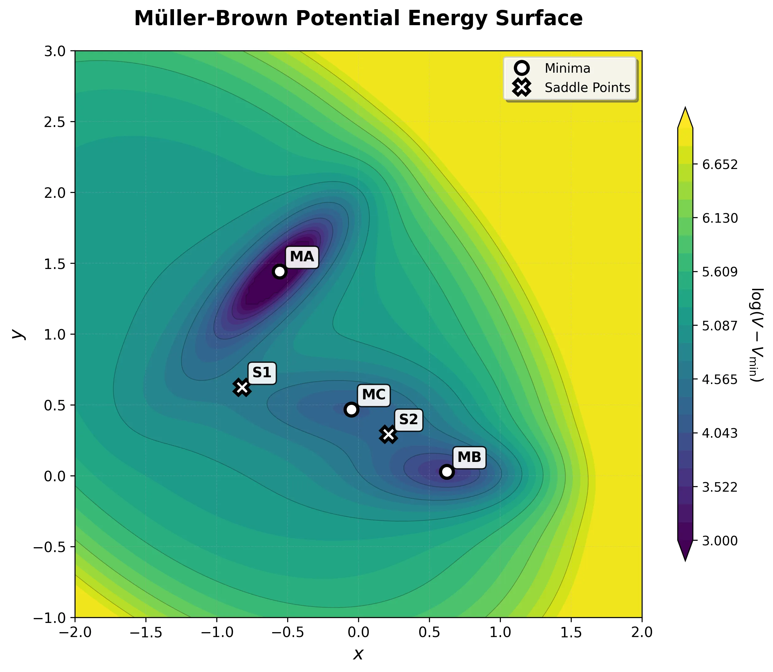
The Resulting Landscape

The Müller-Brown potential energy surface showing the three minima (dark blue regions) and two saddle points.

This simple formula creates a surprisingly rich topography with exactly the features needed to challenge optimization algorithms:

The Key Challenge: Curved Pathways

The path from the deep reactant minimum (MA) to the product minimum (MB) doesn’t go directly over a single barrier. Instead, it follows a curved route:

1. MA → S1 → MC: First transition over a lower barrier into an intermediate basin
2. MC → S2 → MB: Second transition over a slightly higher barrier to the product

This two-step pathway breaks linear interpolation methods. Algorithms that draw a straight line from reactant to product miss both the intermediate minimum and the correct transition states, climbing over much higher energy regions instead.

Why It Works as a Benchmark

The Müller-Brown potential has served as a computational chemistry benchmark for over four decades because of four key characteristics:

Low dimensionality: As a 2D surface, you can visualize the entire landscape and see exactly why algorithms succeed or fail.

Analytical form: Energy and gradient calculations cost virtually nothing, enabling exhaustive testing impossible with quantum mechanical surfaces.

Non-trivial topology: The curved minimum energy path and shallow intermediate minimum challenge sophisticated methods while remaining manageable.

Known ground truth: All minima and saddle points are precisely known, providing unambiguous success metrics.

What makes this particularly valuable is the contrast with other classic potentials. While the Lennard-Jones potential² serves as the benchmark for equilibrium properties with its single energy minimum, Müller-Brown explicitly models reactive landscapes. Its multiple minima and connecting barriers make it the testing ground for algorithms that find reaction paths—the methods that reveal how chemistry actually happens.

Applications Across Decades

The potential has evolved with the field’s changing focus:

1980s-1990s: Testing path-finding methods like Nudged Elastic Band (NEB)³, which creates discrete representations of reaction pathways and optimizes them to find minimum energy paths.

2000s-2010s: Validating Transition Path Sampling (TPS) methods⁴ that harvest statistical ensembles of reactive trajectories rather than single pathways.

2020s: Benchmarking machine learning models and generative approaches that learn to sample transition paths or approximate potential energy surfaces.

Modern Applications in Machine Learning

The rise of machine learning has given the Müller-Brown potential new purpose. Modern Machine Learning Interatomic Potentials (MLIPs)⁵⁶ aim to bridge the gap between quantum mechanical accuracy and classical force field efficiency by training flexible models on expensive quantum chemistry data.

This creates a benchmarking challenge: with countless ML architectures available, how do you objectively compare them? The Müller-Brown potential provides a perfect solution—an exactly known potential energy surface that can generate unlimited, noise-free training data.

This allows researchers to ask fundamental questions:

• How well does a given architecture learn complex, curved surfaces?
• How many training points are needed for acceptable accuracy?
• How does the model behave when extrapolating beyond training data?
• Can it correctly identify minima and saddle points?

The potential has evolved from being a simple model system to serving as a metrological standard—a ruler against which AI learning capacity is measured. Any prediction error is purely due to model limitations, not data quality issues.

These benchmarking principles extend beyond abstract test cases. Real molecular dynamics simulations, such as those studying adatom diffusion on metal surfaces, face similar challenges in understanding energy landscapes and transition pathways. The Müller-Brown potential provides a controlled environment for developing methods that eventually tackle these complex realistic systems.

Extension to Higher Dimensions

The canonical Müller-Brown potential can be extended beyond two dimensions to create more challenging test cases that better reflect real molecular systems. This extensibility demonstrates why it remains such an effective template for computational method development.

Why Higher Dimensions Matter

Real molecules have dozens or hundreds of degrees of freedom, not just two. Understanding how algorithms scale with dimensionality is crucial for practical applications. Higher-dimensional extensions allow researchers to systematically test:

• Algorithm scaling - Does performance degrade gracefully as dimensions increase?
• Model robustness - Do machine learning approaches maintain accuracy in high-dimensional spaces?
• Parallel efficiency - Can massively parallel methods exploit additional dimensions effectively?

Extension Approaches

Harmonic constraints: Add quadratic wells in orthogonal dimensions while preserving the complex 2D landscape⁷:

$$V_{5D}(x_1, x_2, x_3, x_4, x_5) = V(x_1, x_3) + \kappa(x_2^2 + x_4^2 + x_5^2)$$

The parameter $\kappa$ controls constraint strength—small values create nearly flat directions that test algorithmic efficiency.

Collective variables: Define new coordinates that mix multiple dimensions⁸:

$$\tilde{x} = \sqrt{x_1^2 + x_2^2 + \epsilon x_5^2},\quad \tilde{y} = \sqrt{x_3^2 + x_4^2}$$

where $\epsilon \ll 1$. The 5D potential becomes $V_{5D}(\tilde{x}, \tilde{y}) = V(\tilde{x}, \tilde{y})$, embedding the original surface in a higher-dimensional space.

Value for Algorithm Development

This extensibility makes the Müller-Brown potential ideal for systematic testing:

• Progressive complexity: Debug on 2D, then scale to higher dimensions
• Ground truth preservation: Known minima and saddle points remain in the active subspace
• Realistic challenges: Captures the “needle in a haystack” problem of transition state finding while maintaining analytical tractability

These extensions transform a simple 2D benchmark into a scalable testbed for modern computational methods, probing specific challenges in high-dimensional optimization.

Implementation in PyTorch

Let’s implement the Müller-Brown potential in PyTorch. A practical implementation needs to handle batch processing, support both analytical and automatic differentiation, and be optimized for performance.

Core Implementation

import torch
import torch.nn as nn
from torch import Tensor

class MuellerBrownPotential(nn.Module):
    """Müller-Brown potential with JIT-compiled force calculations."""

    def __init__(
        self,
        device: str | torch.device = "cpu",
        dtype: torch.dtype = torch.float64,
        use_autograd: bool = False
    ):
        super().__init__()
        self.use_autograd = use_autograd

        # Standard Müller-Brown parameters
        self.register_buffer(
            "A", torch.tensor([-200.0, -100.0, -170.0, 15.0],
                             device=device, dtype=dtype)
        )
        self.register_buffer(
            "a", torch.tensor([-1.0, -1.0, -6.5, 0.7],
                             device=device, dtype=dtype)
        )
        self.register_buffer(
            "b", torch.tensor([0.0, 0.0, 11.0, 0.6],
                             device=device, dtype=dtype)
        )
        self.register_buffer(
            "c", torch.tensor([-10.0, -10.0, -6.5, 0.7],
                             device=device, dtype=dtype)
        )
        self.register_buffer(
            "x_centers", torch.tensor([1.0, 0.0, -0.5, -1.0],
                                    device=device, dtype=dtype)
        )
        self.register_buffer(
            "y_centers", torch.tensor([0.0, 0.5, 1.5, 1.0],
                                    device=device, dtype=dtype)
        )

    def forward(self, coordinates: Tensor) -> Tensor:
        """Compute potential energy."""
        return _calculate_potential(
            coordinates, self.A, self.a, self.b, self.c,
            self.x_centers, self.y_centers
        )

    def force(self, coordinates: Tensor) -> Tensor:
        """Compute forces (negative gradient)."""
        if self.use_autograd:
            coordinates = coordinates.requires_grad_(True)
            potential = self.forward(coordinates)
            grad = torch.autograd.grad(potential.sum(), coordinates)[0]
            return -grad
        else:
            return _calculate_force(
                coordinates, self.A, self.a, self.b, self.c,
                self.x_centers, self.y_centers
            )

The implementation uses register_buffer to store parameters, ensuring they move with the model to the appropriate device. The use_autograd flag switches between analytical and automatic differentiation.

JIT Compilation for Performance

PyTorch’s JIT compiler optimizes the mathematical operations for better performance:

@torch.jit.script
def _calculate_potential(coordinates: Tensor, A: Tensor, a: Tensor,
                        b: Tensor, c: Tensor, x_centers: Tensor,
                        y_centers: Tensor) -> Tensor:
    """JIT-scripted potential energy calculation."""
    coords = coordinates.view(-1, 2)
    x, y = coords[:, 0], coords[:, 1]
    dx = x.unsqueeze(-1) - x_centers
    dy = y.unsqueeze(-1) - y_centers

    potential = torch.sum(
        A * torch.exp(a * dx**2 + b * dx * dy + c * dy**2),
        dim=-1
    )
    return potential.view(coordinates.shape[:-1])

@torch.jit.script
def _calculate_force(coordinates: Tensor, A: Tensor, a: Tensor,
                    b: Tensor, c: Tensor, x_centers: Tensor,
                    y_centers: Tensor) -> Tensor:
    """JIT-scripted force calculation."""
    coords = coordinates.view(-1, 2)
    x, y = coords[:, 0], coords[:, 1]
    dx = x.unsqueeze(-1) - x_centers
    dy = y.unsqueeze(-1) - y_centers

    exp_terms = torch.exp(a * dx**2 + b * dx * dy + c * dy**2)
    A_exp = A * exp_terms

    grad_x = torch.sum(A_exp * (2 * a * dx + b * dy), dim=-1)
    grad_y = torch.sum(A_exp * (b * dx + 2 * c * dy), dim=-1)

    forces = torch.stack([-grad_x, -grad_y], dim=-1)
    new_shape = list(coordinates.shape[:-1]) + [2]
    return forces.view(new_shape)

JIT compilation eliminates Python overhead, optimizes memory usage, and enables better vectorization.

Performance: Analytical vs. Automatic Differentiation

A key design decision is whether to use analytical derivatives or automatic differentiation. I benchmarked both approaches on a 2020 MacBook Pro using PyTorch 2.0.1:

Throughput comparison showing analytical derivatives consistently outperform autograd by 3-10x.

Per-particle computation time. Analytical derivatives maintain sub-microsecond performance for large systems.

The results show analytical derivatives consistently outperform autograd by 3-10x across all problem sizes. This advantage comes from avoiding the computational graph overhead inherent in automatic differentiation.

When to use each approach:

• Analytical: Best for molecular dynamics where forces are computed millions of times. The speedup directly reduces simulation time.
• Autograd: Better for machine learning applications where convenience and guaranteed correctness often outweigh performance costs during development.

Molecular Dynamics Simulations

To demonstrate the PyTorch implementation in action, we performed Langevin dynamics simulations in different energy basins. These simulations reveal how particles behave when confined to different regions of the potential energy surface.

Simulation Parameters

We ran 3600 time steps with a 0.01 time unit step size, using a friction coefficient of 1.0 and temperature of 25.0 in reduced units. The simulations started from equilibrium positions within each basin and show the characteristic thermal fluctuations around local minima.

Basin MA: Deep Reactant Minimum

The deepest energy well (-146.70 kJ/mol) shows highly constrained motion due to the steep energy barriers surrounding it.

Basin MB: Product Minimum

The product minimum (-108.17 kJ/mol) shows intermediate behavior between the deep reactant well and shallow intermediate basin.

Transition Example

Running a longer simulation demonstrates transitions between basins.

Integration with Modern Workflows

The PyTorch implementation integrates naturally with machine learning workflows. It can serve as a component in larger computational graphs, enable gradient-based optimization, and bridge classical molecular simulation with deep learning approaches.

For readers interested in broader molecular ML applications, this implementation pairs well with other molecular representation methods. The Coulomb matrix approach offers complementary perspectives on encoding molecular structure, while the Kabsch algorithm provides essential tools for structural alignment.

The complete implementation is available on GitHub⁹¹⁰¹¹, including benchmarking scripts, visualization tools, and examples for optimization and molecular dynamics.

Conclusion

The Müller-Brown potential exemplifies how a well-designed benchmark can evolve with a field. Born from 1970s computational constraints, it provided a simple way to test algorithms when quantum chemistry calculations were expensive. Its clever design—simple enough to compute instantly, complex enough to break naive approaches—made it invaluable for algorithm development.

Today, it serves new purposes in the machine learning era. The PyTorch implementation shows how classic benchmarks adapt to modern frameworks. The 3-10x performance advantage of analytical derivatives remains important for intensive simulations, while PyTorch’s flexibility enables integration with machine learning workflows.

The potential’s evolution from practical necessity to pedagogical tool to machine learning benchmark demonstrates the value of foundational test cases. As computational chemistry continues evolving, reliable standards like the Müller-Brown potential become even more important for rigorous method development and comparison.