Introduction
When working with machine learning in chemistry, one of the first challenges you encounter is how to represent molecules in a way that algorithms can understand. You can’t just feed raw atomic coordinates into a model. The representation needs to be invariant to rotation, translation, and atom ordering, since these operations don’t change the molecule’s fundamental properties.
The Coulomb matrix, introduced by Rupp et al. in 2012 [1], provides a straightforward solution to this problem. While newer methods have largely superseded it for practical applications, the Coulomb matrix remains an excellent starting point for understanding how molecular descriptors work.
The key insight is simple: we encode pairwise relationships between atoms in a way that captures the essential physics while maintaining the required invariances.
The Coulomb Matrix: Theory and Intuition
The Coulomb matrix encodes molecular structure in a symmetric $N \times N$ matrix, where $N$ is the number of atoms. Each element $C_{ij}$ is defined as:
$$ C_{ij} = \begin{cases} 0.5 Z_i^{2.4} & \text{if } i = j, \\ \frac{Z_i Z_j}{|\mathbf{R}_i - \mathbf{R}_j|} & \text{if } i \neq j, \end{cases} $$
Here, $Z_i$ is the atomic number of atom $i$, and $\mathbf{R}_i$ is its position in 3D space. The diagonal elements ($0.5 Z_i^{2.4}$) represent atomic self-energies, derived from fitting atomic numbers to experimental data. The off-diagonal elements mimic Coulombic interactions between atoms. They’re inversely proportional to distance, just like electrostatic potential energy [3].
This construction gives us several useful properties:
- Rotation and translation invariant: Only relative distances matter
- Symmetric: $C_{ij} = C_{ji}$, which is physically sensible
- Size-extensive: Larger molecules have larger matrix elements
- Captures 3D structure: Nearby atoms have larger interaction terms
While more sophisticated methods exist today [2], the Coulomb matrix’s simplicity makes it ideal for understanding the fundamentals of molecular representation.
Hands-on Example: Bicyclobutane
Let’s calculate the Coulomb matrix for bicyclobutane, a strained but stable four-membered ring system. This example will show you exactly how the theory translates to practice.

I’ll use Python with the Atomic Simulation Environment (ase) for molecular structure [4] and dscribe for the Coulomb matrix calculation [2]:
from ase.build import molecule
from ase.visualize import view

# Load the bicyclobutane structure
bicyclobutane = molecule('bicyclobutane')

# Optional: visualize the structure
view(bicyclobutane, viewer='x3d')

Now we calculate the Coulomb matrix using DScribe:
from dscribe.descriptors import CoulombMatrix

# Set up the descriptor
cm = CoulombMatrix(n_atoms_max=len(bicyclobutane))

# Calculate and reshape into matrix form
cm_bicyclobutane = cm.create(bicyclobutane)
cm_bicyclobutane = cm_bicyclobutane.reshape(len(bicyclobutane), len(bicyclobutane))
Visualizing the Results
The Coulomb matrix can be visualized as a heatmap. Let’s look at both the raw matrix and its logarithm:
import matplotlib.pyplot as plt
import numpy as np

# Raw Coulomb matrix
plt.figure(figsize=(8, 8), dpi=150)
plt.imshow(cm_bicyclobutane, cmap='coolwarm')
plt.colorbar(label='Magnitude')
plt.title('Coulomb Matrix for Bicyclobutane')
plt.show()

The raw matrix shows clear patterns:
- Large diagonal elements: Carbon atoms (Z=6) dominate due to their higher atomic numbers
- Smaller off-diagonal elements: Represent pairwise interactions
- Minimal hydrogen contribution: Hydrogen atoms (Z=1) have much smaller values
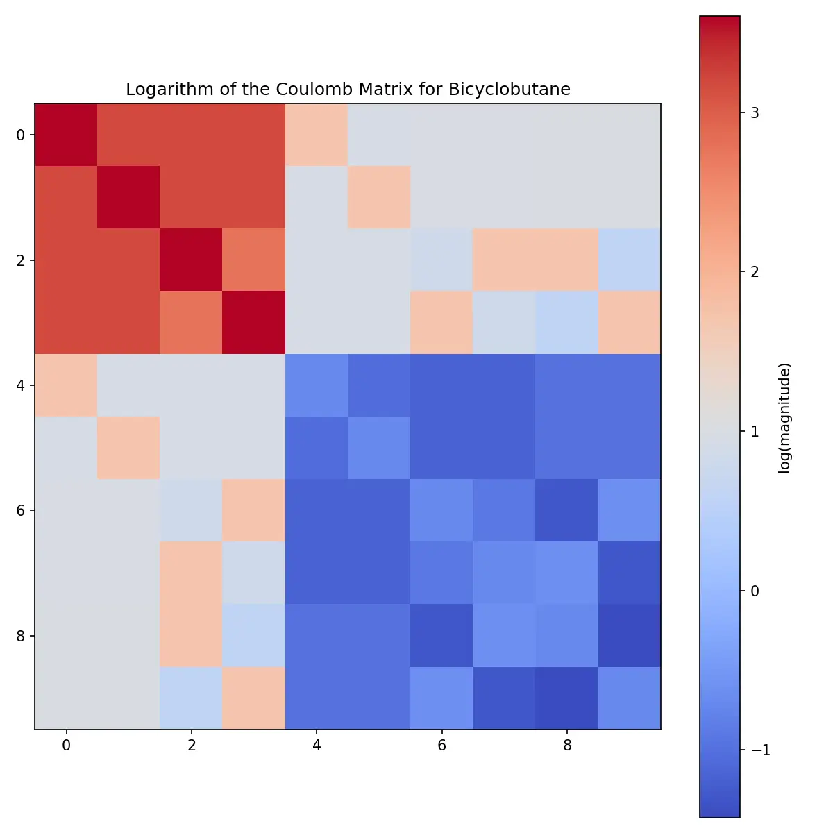
For better visualization of the structure, the logarithm reveals more detail:
plt.figure(figsize=(8, 8), dpi=150)
plt.imshow(np.log(cm_bicyclobutane), cmap='coolwarm')
plt.colorbar(label='log(Magnitude)')
plt.title('Log Coulomb Matrix for Bicyclobutane')
plt.show()

Eigenvalue Analysis
The eigenvalues of the Coulomb matrix provide another perspective on molecular structure:


These eigenvalues are often used as features themselves, providing a more compact representation than the full matrix.
Practical Limitations
The Coulomb matrix has significant limitations that explain why it’s been largely superseded by modern methods. Understanding these constraints is crucial for knowing when and how to use this descriptor.
The Size Problem
Every molecule must be represented by the same size matrix, which creates several issues:
- Padding overhead: Small molecules get padded with zeros up to the maximum size
- Quadratic scaling: An $N$-atom molecule requires $N^2$ features
- Fixed maximum size: You can’t represent molecules larger than your preset limit
- Inefficient storage: Most elements are zero for small molecules in large matrices
For a dataset ranging from 5-atom to 50-atom molecules, every molecule needs a 50x50 matrix. That’s 2,500 features, most of which are zero for smaller molecules.
Permutation Sensitivity
Despite being called “invariant,” the Coulomb matrix can actually change if you reorder the atoms in your input file. The standard solution is to sort atoms by the L2 norm of their matrix rows, but this introduces its own problems:
- Symmetry breaking: Equivalent atoms might be ordered differently
- Numerical instability: Small coordinate changes can flip the ordering
- Loss of chemical intuition: The sorted order doesn’t reflect meaningful chemistry
Interestingly, some studies suggest that adding controlled noise to create multiple permutations can actually improve machine learning performance [5].
Limited Scope
The Coulomb matrix works well only for specific types of systems:
- Small molecules: Performance degrades for large systems due to size scaling
- Gas-phase: Not suitable for periodic systems like crystals or surfaces
- Single conformations: Each 3D structure gets its own matrix
- Non-reactive: Doesn’t capture bond-breaking or formation
For periodic systems, you’d need specialized variants like the Ewald sum matrix [6].
Why Learn It Anyway?
Given these limitations, why spend time understanding the Coulomb matrix? Several reasons:
Educational value: It’s conceptually straightforward and provides excellent intuition for how molecular descriptors work. The mathematical formulation is simple enough to implement from scratch.
Historical importance: Many subsequent methods build on ideas first explored with Coulomb matrices. Understanding this foundation helps you appreciate why newer methods were developed.
Benchmarking: It remains useful as a baseline method for comparing new descriptors on small molecular datasets.
Proof of concept: For exploratory work on small, well-defined datasets, the Coulomb matrix can still provide quick insights.
If you’re working on practical problems with larger datasets or diverse molecular sizes, consider modern alternatives like graph neural networks, descriptors from DScribe’s extended library, or learned representations from transformer models.
Putting It in Context
To see the Coulomb matrix applied to real problems, I’ve written a detailed guide using it for molecular classification:
- Coulomb Matrix Eigenvalues: Can You Hear the Shape of a Molecule?: A comprehensive analysis of alkane isomers, from unsupervised clustering limits to supervised classification successes.
For comparison with modern approaches, check out my post on 3D conformer generation with the GEOM dataset, which showcases more sophisticated molecular representations. For technical specifications and benchmarks, see the GEOM dataset card.
The Coulomb matrix may be dated, but it remains an excellent entry point into the world of molecular machine learning. Once you understand its strengths and limitations, you’ll be better equipped to appreciate why the field has moved toward more sophisticated approaches.
Have questions about molecular descriptors or want to discuss other approaches to molecular machine learning? I’d be happy to explore these topics further.
References
- [1]: M. Rupp, A. Tkatchenko, K.-R. Müller, and O. A. von Lilienfeld, “Fast and Accurate Modeling of Molecular Atomization Energies with Machine Learning,” Physical Review Letters, 108(5), 058301 (2012). https://doi.org/10.1103/PhysRevLett.108.058301 arXiv:1109.2618
- [2] L. Himanen, M. O. J. Jäger, E. V. Morooka, F. F. Canova, Y. S. Ranawat, D. Z. Gao, P. Rinke, and A. S. Foster, “DScribe: Library of descriptors for machine learning in materials science,” Computer Physics Communications, 247, 106949 (2020). https://doi.org/10.1016/j.cpc.2019.106949 arXiv:1904.08875
- [3] J. Schrier, “Can one hear the shape of a molecule (from its Coulomb matrix eigenvalues)?,” Journal of Chemical Information and Modeling, 60(8), 3804-3811 (2020). https://doi.org/10.1021/acs.jcim.0c00631
- [4] A. H. Larsen, J. J. Mortensen, J. Blomqvist, I. E. Castelli, R. Christensen, M. Dułak, J. Friis, M. N. Groves, B. Hammer, C. Hargus, E. D. Hermes, P. C. Jennings, P. B. Jensen, J. Kermode, J. R. Kitchin, E. L. Kolsbjerg, J. Kubal, K. Kaasbjerg, S. Lysgaard, J. B. Maronsson, T. Maxson, T. Olsen, L. Pastewka, A. Peterson, C. Rostgaard, J. Schiøtz, O. Schütt, M. Strange, K. S. Thygesen, T. Vegge, L. Vilhelmsen, M. Walter, Z. Zeng, and K. W. Jacobsen, “The Atomic Simulation Environment - A Python library for working with atoms,” J. Phys.: Condens. Matter, 29, 273002 (2017). https://doi.org/10.1088/1361-648X/aa680e documentation
- [5] G. Montavon, K. Hansen, S. Fazli, M. Rupp, F. Biegler, A. Ziehe, A. Tkatchenko, A. Lilienfeld, and K.-R. Müller, “Learning invariant representations of molecules for atomization energy prediction,” Advances in Neural Information Processing Systems, 25 (2012). Available online: https://proceedings.neurips.cc/paper_files/paper/2012/file/115f89503138416a242f40fb7d7f338e-Paper.pdf
- [6] F. Faber, A. Lindmaa, O. A. von Lilienfeld, and R. Armiento, “Crystal structure representations for machine learning models of formation energies,” International Journal of Quantum Chemistry, 115(16), 1094-1101 (2015). https://doi.org/10.1002/qua.24917