Modern PyTorch Techniques for VAEs: A Hands-On Tutorial

What is a Variational Autoencoder?

A Variational Autoencoder (VAE) is a type of generative model, meaning its primary purpose is to learn the underlying structure of a dataset so it can generate new, similar data.

Whether the data is images, raw audio clips, or 2D graphs of drug-like molecules, a VAE aims to capture the essential features that define the data distribution. Once trained, it should be able to create entirely new samples that resemble the training data but are not direct copies.

Introduced by Kingma and Welling in 2013 (Auto-Encoding Variational Bayes), VAEs are powerful tools for:

• Generation: Creating new data (images, music, text).
• Dimensionality Reduction: Compressing data into a much smaller, meaningful representation (a “latent space”).
• Imputation: Intelligently filling in missing data (e.g., denoising images).

Importantly, they aim to provide a structured and continuous latent space, which allows for smooth interpolation between data points and meaningful manipulations of generated samples (think: optimization).

The Core Idea: Learning to Generate

The VAE is built on a key assumption: our complex, high-dimensional data (like a $28 \times 28$ pixel image, $\mathbf{x}$) is actually generated by some simpler, low-dimensional, unobserved variable (a “latent” variable, $\mathbf{z}$).

A Physical Metaphor: Water Molecules and Phase Diagrams

Consider a glass of water. At the microscopic level, you have more than $10^{24}$ $\text{H}_2\text{O}$ molecules bouncing around in an incredibly high-dimensional space. Each molecule has position, velocity, and interactions with its neighbors, computationally intractable to track directly. Yet we can describe the macroscopic behavior of all these molecules using just two simple variables: temperature and pressure. These two dimensions create a “phase diagram” that tells us whether our water will be ice, liquid, or vapor. The temperature and pressure are “latent variables” that capture the essential physics governing this complex molecular dance.

A VAE makes the same assumption: complex data (like images) emerges from simpler underlying factors. A handwritten digit might be generated by latent factors like “pen thickness,” “writing angle,” “digit style,” and “size,” a much simpler description than tracking all 784 pixel values independently.

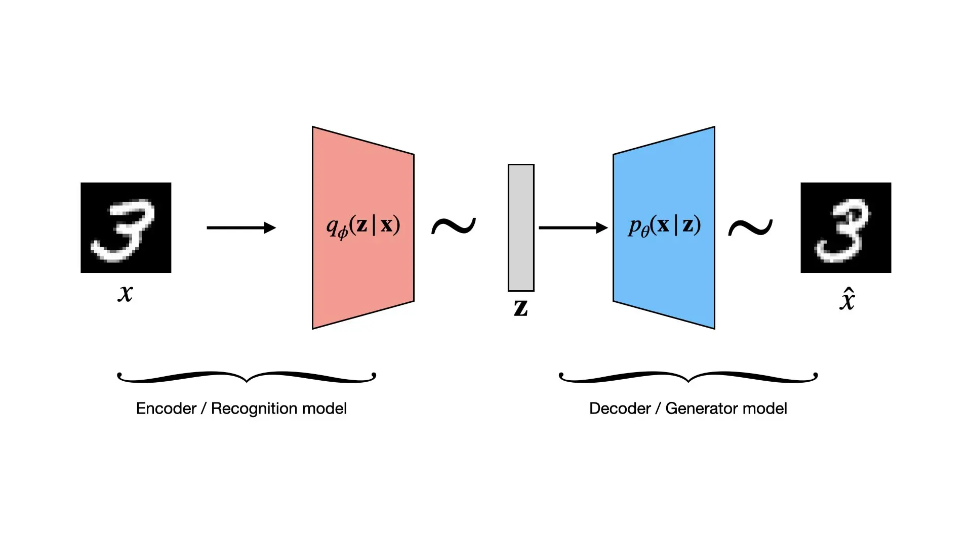
The VAE learns two functions: one that maps from complex data ($\mathbf{x}$) to these descriptive factors ($\mathbf{z}$), and another that maps from these factors back to the data. It accomplishes this with two main components, typically implemented as neural networks:

1. The Encoder (Recognition Model)

This network takes a complex data point $\mathbf{x}$ (an image) and determines the “knob settings” $\mathbf{z}$ that could explain or generate it. This allows us to compress or understand the data.

$$q_{\phi}(\mathbf{z} | \mathbf{x})$$

It’s like examining a container of molecules and summarizing their complex arrangement into key parameters like temperature and pressure.

Crucially, the encoder doesn’t output the latent vector $\mathbf{z}$ directly. Instead, it outputs the parameters of a probability distribution (a simple Gaussian) that describes $\mathbf{z}$.

For each input $\mathbf{x}$, the encoder network outputs:

• A vector of means, $\mathbf{\mu}$
• A vector of standard deviations, $\mathbf{\sigma}$

These parameters define our approximation $q_{\phi}(\mathbf{z} | \mathbf{x}) = \mathcal{N}(\mathbf{z} \mid \mathbf{\mu}, \mathbf{\sigma}^2\mathbf{I})$. We then sample from this distribution to get the $\mathbf{z}$ that we feed to the decoder. This probabilistic step is what forces the latent space to be continuous and structured. It forces similar inputs to map to nearby regions in latent space, enabling smooth interpolation and generation.

2. The Decoder (Generative Model)

This network learns the “generative process.” It takes a simple latent vector $\mathbf{z}$ and reconstructs the complex data $\mathbf{x}$. This allows us to generate new data by feeding it a random $\mathbf{z}$ and observing what image $\mathbf{x}$ it produces.

$$p_{\theta}(\mathbf{x} | \mathbf{z})$$

The decoder reverses the encoder: it takes the simple latent representation and “paints” the full, complex image from it. It’s like taking temperature and pressure values and producing a detailed arrangement of water molecules consistent with those conditions. The goal is to reproduce the exact input as closely as possible.

After training, we have two networks that can be used for a variety of purposes:

• Generation: If the latent space is well-structured, we can sample random $\mathbf{z}$ vectors from a simple distribution (like a standard normal) and feed them into the Decoder to generate new images. This is particularly useful for searching for data points with desired properties, like in drug discovery, where we might want to generate molecules with specific characteristics.
• Compression: The Encoder can compress complex data into a low-dimensional latent space, which can be useful for visualization or as a feature extractor for other tasks.

The “Variational” Problem (and its Solution)

Ideally, for a given input $\mathbf{x}$, we’d like to find the true distribution of latent variables that could have created it, $p_{\theta}(\mathbf{z}|\mathbf{x})$. Unfortunately, calculating this “true posterior” is mathematically intractable.

Why? Let’s examine Bayes’ theorem:

$$p_{\theta}(\mathbf{z} | \mathbf{x}) = \frac{p_{\theta}(\mathbf{x} | \mathbf{z}) p_{\theta}(\mathbf{z})}{p_{\theta}(\mathbf{x})}$$

Breaking down each component:

• $p_{\theta}(\mathbf{x} | \mathbf{z})$ is our decoder, which is straightforward to compute given our likelihood model.
• $p_{\theta}(\mathbf{z})$ is our prior over latent variables, typically a simple distribution like a standard normal, making it easy to compute.
• $p_{\theta}(\mathbf{x})$ is the marginal likelihood of the data. And here lies the problem. It requires integrating over all possible latent variables that could have generated $\mathbf{x}$: $$p_{\theta}(\mathbf{x}) = \int p_{\theta}(\mathbf{x} | \mathbf{z}) p_{\theta}(\mathbf{z}) d\mathbf{z}$$ It is the normalization factor that ensures the posterior is a valid probability distribution (i.e., sums to 1 over all $\mathbf{z}$).

This integral is intractable because it involves integrating over a high-dimensional latent space with a complex likelihood function. No closed-form solution exists, and numerical integration is computationally prohibitive.

This is where the “variational” approach provides the solution. Instead of learning the true posterior, we’ll learn an encoder, $q_{\phi}(\mathbf{z} | \mathbf{x})$, that serves as a variational approximation to this intractable true distribution. The VAE’s training process optimizes this approximation to be as accurate as possible, pushing this learned distribution closer to the true posterior.

The VAE Objective: A Balancing Act

To get these two networks (parameterized by $\theta$ and $\phi$) to work together, we train them jointly with a special loss function. This objective has two parts that balance two different goals:

1. Reconstruction Loss

$$E_{q_{\phi}(\mathbf{z} | \mathbf{x})}[\log p_{\theta}(\mathbf{x} | \mathbf{z})]$$

This term asks: “How well can we reconstruct our original image?” It forces the VAE to be good at its job. The process goes:

1. Take an input point $\mathbf{x}$.
2. Use the Encoder to get its latent representation $\mathbf{z} \sim q_{\phi}(\mathbf{z} | \mathbf{x})$.
3. Use the Decoder to generate a new image $\mathbf{x}’$ from $\mathbf{z}$, $\mathbf{x}’ \sim p_{\theta}(\mathbf{x} | \mathbf{z})$.
4. Compare $\mathbf{x}$ and $\mathbf{x}’$.

The reconstruction loss measures the difference between the original and the reconstructed image.

• For continuous inputs (like general images), this is often Mean Squared Error (MSE).
• For discrete inputs (like MNIST, where pixels are 0 or 1), we use Binary Cross-Entropy (BCE). We treat each pixel as an independent Bernoulli random variable (either on or off). The decoder outputs the logits (log-probabilities) for each pixel, and the BCE loss (e.g., F.binary_cross_entropy_with_logits) is the numerically stable way to compute the negative log-likelihood.
• More generally, you can output parameters of a desired output distribution. What if you wanted a mixture of Gaussians? The decoder could output the means, variances, and mixture weights, and you could compute the negative log-likelihood accordingly.

This loss pushes the encoder to produce useful $\mathbf{z}$ vectors and pushes the decoder to learn how to interpret them accurately.

2. The KL Divergence (The Regularizer)

$$D_{KL}(q_{\phi}(\mathbf{z} | \mathbf{x}) || p_{\theta}(\mathbf{z}))$$

On its own, the reconstruction loss might “cheat.” The encoder could learn to map every image to a different, specific point in the latent space, essentially “memorizing” the data. This would be great for reconstruction but terrible for generation, as the space between these points would be meaningless.

The KL divergence term fixes this. It’s a regularizer that forces the latent space to be organized and smooth.

We force the encoder’s output, $q_{\phi}(\mathbf{z} | \mathbf{x})$, to be close to a simple, predefined prior distribution, $p_{\theta}(\mathbf{z})$. This prior is almost always a standard normal distribution, partly because it’s mathematically convenient and easy to sample from afterward, but also because it encourages the latent space to be well-behaved.

This regularization term acts as a penalty, measuring how much the encoder’s output distribution diverges from the simple prior. By minimizing this KL divergence, we encourage the model to:

• Avoid overfitting by preventing the encoder from memorizing specific locations for each input
• Create meaningful clusters where similar inputs map to nearby regions in the latent space
• Maintain continuity so that points close together in latent space (like different variations of the digit “7”) decode into visually similar outputs

This smooth, structured latent space is what enables generation: we can sample random points from our prior distribution and decode them into realistic new data.

Ultimately, the optimizer finds a balance between these two objectives: reconstructing the data well while keeping the latent space organized and regularized.

The Reparameterization Trick: Making it All Trainable

We have a problem. The training process requires sampling:

1. Encoder produces $\mathbf{\mu}$ and $\mathbf{\sigma}$.
2. We sample $\mathbf{z} \sim \mathcal{N}(\mathbf{\mu}, \mathbf{\sigma}^2\mathbf{I})$.
3. Decoder uses $\mathbf{z}$ to reconstruct $\mathbf{x}’$.
4. We calculate the loss.

The “sampling” step is a random, non-differentiable operation. We can’t backpropagate the reconstruction loss from the decoder through this random node to update the encoder’s weights.

The reparameterization trick solves this by reframing the sampling process. Instead of sampling $\mathbf{z}$ from the encoder’s distribution, we create $\mathbf{z}$ deterministically like this:

1. Sample a random noise vector $\mathbf{\epsilon}$ from a simple, fixed distribution (e.g., the standard normal $\mathcal{N}(\mathbf{0}, \mathbf{I})$).
2. Compute $\mathbf{z}$ as: $\mathbf{z} = \mathbf{\mu} + \mathbf{\sigma} \odot \mathbf{\epsilon}$

This simple change moves the randomness “outside” the network. The gradient can now flow deterministically from $\mathbf{z}$ back through the $\mathbf{\mu}$ and $\mathbf{\sigma}$ nodes to the encoder network. This is the key engineering insight that allows us to train the entire model end-to-end with standard backpropagation.

Where Does This Objective Come From? (The Math)

This two-part loss function isn’t just a clever heuristic. It’s derived directly from trying to maximize the marginal likelihood of the data, $\log p_{\theta}(\mathbf{x})$.

For a single data point $\mathbf{x}^{(i)}$, we can write: $$\log p_{\theta}(\mathbf{x}^{(i)}) = D_{KL}(q_\phi(\mathbf{z} | \mathbf{x}^{(i)}) || p_{\theta}(\mathbf{z} | \mathbf{x}^{(i)})) + \mathcal{L}(\theta, \phi; \mathbf{x}^{(i)})$$

• The first term is the KL divergence between our encoder’s approximation and the (intractable) true posterior. This is non-negative but unfortunately we can’t compute it.
• The second term, $\mathcal{L}$, is the Variational Lower Bound (also known as the Evidence Lower Bound, or ELBO). Since the KL term is $\ge 0$, we know that $\log p_{\theta}(\mathbf{x}^{(i)}) \ge \mathcal{L}$.

By maximizing this lower bound $\mathcal{L}$, we push up the “floor” on the true likelihood of our data. This is a problem we can solve.

When we expand this $\mathcal{L}$ term, we get our famous two-part objective:

$$\mathcal{L}(\theta, \phi; \mathbf{x}^{(i)}) = E_{q_{\phi}(\mathbf{z} | \mathbf{x}^{(i)})}[\log p_{\theta}(\mathbf{x}^{(i)} | \mathbf{z})] - D_{KL}(q_\phi(\mathbf{z} | \mathbf{x}^{(i)}) || p_{\theta}(\mathbf{z}))$$

• Term 1: The expected log-likelihood of reconstructing $\mathbf{x}^{(i)}$ from $\mathbf{z}$. Maximizing this is the same as minimizing the Reconstruction Loss.
• Term 2: The negative KL divergence between our encoder and the simple prior. Maximizing this is the same as minimizing the KL Divergence Loss.

Thus, the VAE’s objective balances these two critical goals: faithfully reconstructing the data while maintaining a simple, regularized latent structure that is useful for generation.

From ELBO to Practical Loss

Remember, our goal is to maximize the ELBO:

$$\mathcal{L}(\theta, \phi; \mathbf{x}) = E_{q_{\phi}(\mathbf{z} | \mathbf{x})}[\log p_{\theta}(\mathbf{x} | \mathbf{z})] - D_{KL}(q_\phi(\mathbf{z} | \mathbf{x}) || p_{\theta}(\mathbf{z}))$$

Since deep learning libraries are built to minimize a loss function, we simply flip the sign and minimize the negative ELBO ($-\mathcal{L}$).

This gives us our final, practical loss function:

$$\text{Loss} = -\mathcal{L} = -E_{q_{\phi}(\mathbf{z} | \mathbf{x})}[\log p_{\theta}(\mathbf{x} | \mathbf{z})] + D_{KL}(q_\phi(\mathbf{z} | \mathbf{x}) || p_{\theta}(\mathbf{z}))$$

This is the function you actually implement. Minimizing this loss achieves both of our goals:

1. It minimizes the Reconstruction Loss (which is the same as maximizing the log-likelihood).
2. It minimizes the KL Divergence, forcing the encoder to match the prior.

Modern PyTorch VAE Implementation

Now that we understand the VAE architecture and objective, let’s implement a modern VAE in PyTorch. I’ll focus primarily on the model and loss function here, though the full code is available on GitHub.

My VAE implementation uses an output dataclass and a VAE class extending nn.Module.

"""Variational Autoencoder (VAE) model implementation."""

from dataclasses import dataclass

import torch
import torch.nn as nn
import torch.nn.functional as F


def get_activation(activation: str) -> nn.Module:
    """Get activation function by name."""
    activation_lower = activation.lower()
    ACTIVATION_MAP = {
        "relu": nn.ReLU(),
        "tanh": nn.Tanh(),
        "sigmoid": nn.Sigmoid(),
        "leaky_relu": nn.LeakyReLU(),
        "elu": nn.ELU(),
        "gelu": nn.GELU(),
    }
    if activation_lower not in ACTIVATION_MAP:
        supported = ", ".join(ACTIVATION_MAP.keys())
        raise ValueError(
            f"Unsupported activation '{activation}'. Supported: {supported}"
        )
    return ACTIVATION_MAP[activation_lower]


@dataclass
class VAEConfig:
    """VAE model configuration specifying architecture and behavior."""

    hidden_dim: int
    latent_dim: int

    input_shape: tuple[int, int, int] = (1, 28, 28)  # Default: MNIST
    activation: str = "tanh"  # Default: tanh, what was used in the original VAE paper
    use_softplus_std: bool = False  # Whether to use softplus for std parameterization
    n_samples: int = 1  # Number of latent samples per input during training


@dataclass
class VAEOutput:
    """VAE forward pass output containing all relevant tensors and optional losses."""

    x_logits: torch.Tensor
    z: torch.Tensor
    mu: torch.Tensor
    std: torch.Tensor

    x_recon: torch.Tensor | None = None
    loss: torch.Tensor | None = None
    loss_recon: torch.Tensor | None = None
    loss_kl: torch.Tensor | None = None


class VAE(nn.Module):
    """Variational Autoencoder with support for deterministic and probabilistic reconstruction."""

    DEFAULT_EPS = 1e-8

    def __init__(self, config: VAEConfig) -> None:
        """Initialize VAE with given configuration.

        Args:
            config: VAE configuration specifying architecture and behavior
        """
        super().__init__()
        self.config = config

        # Build encoder: input -> hidden -> latent parameters (mu, sigma)
        self.encoder = nn.Sequential(
            nn.Flatten(),
            nn.Linear(
                int(torch.prod(torch.tensor(config.input_shape))), config.hidden_dim
            ),
            get_activation(config.activation),
            nn.Linear(config.hidden_dim, config.latent_dim * 2),
        )

        # Build decoder: latent -> hidden -> reconstructed input
        self.decoder = nn.Sequential(
            nn.Linear(config.latent_dim, config.hidden_dim),
            get_activation(config.activation),
            nn.Linear(
                config.hidden_dim, int(torch.prod(torch.tensor(config.input_shape)))
            ),
            nn.Unflatten(1, config.input_shape),
        )

    def encode(self, x: torch.Tensor) -> tuple[torch.Tensor, torch.Tensor]:
        """Encode input to latent distribution parameters."""
        encoder_output = self.encoder(x)
        mu, sigma = torch.chunk(encoder_output, 2, dim=-1)
        return mu, sigma

    def decode(self, z: torch.Tensor) -> torch.Tensor:
        """Decode latent representation to reconstruction logits"""
        return self.decoder(z)

    def reparameterize(self, mu: torch.Tensor, std: torch.Tensor) -> torch.Tensor:
        """Apply reparameterization trick for differentiable sampling."""
        epsilon = torch.randn_like(std)
        return mu + std * epsilon

    def forward(
        self,
        x: torch.Tensor,
        compute_loss: bool = True,
        reconstruct: bool = False,
        eps: float = DEFAULT_EPS,
    ) -> VAEOutput:
        """Forward pass through the VAE.

        Args:
            x: Input tensor of shape (batch_size, *input_shape)
            compute_loss: Whether to compute VAE loss components
            reconstruct: Whether to return reconstructions or distributions
            eps: Small epsilon value for numerical stability

        Returns:
            VAEOutput containing all relevant tensors and optionally computed losses
        """
        # Prepare input for multiple sampling if needed
        x_expanded = self._expand_for_sampling(x) if self.config.n_samples > 1 else x

        # Encode and sample from latent space
        mu, sigma = self.encode(x)
        std = self._sigma_to_std(sigma, eps=eps)
        mu_expanded, std_expanded = self._expand_latent_params(mu, std)
        z = self.reparameterize(mu_expanded, std_expanded)

        # Decode latent samples
        x_logits = self.decode(z)

        # Create output object
        output = VAEOutput(
            x_logits=x_logits,
            z=z,
            mu=mu,
            std=std,
            x_recon=torch.sigmoid(x_logits) if reconstruct else None,
        )

        # Compute losses if requested
        if compute_loss:
            loss, loss_recon, loss_kl = self._compute_loss(
                x_expanded, x_logits, mu, sigma, std
            )
            output.loss = loss
            output.loss_recon = loss_recon
            output.loss_kl = loss_kl

        return output

    # ==================== Helper Methods ====================

    def _sigma_to_std(
        self, sigma: torch.Tensor, eps: float = DEFAULT_EPS
    ) -> torch.Tensor:
        """Convert sigma parameter to standard deviation."""
        if self.config.use_softplus_std:
            return F.softplus(sigma) + eps
        else:
            return torch.exp(0.5 * sigma)  # sigma represents log-variance

    def _expand_for_sampling(self, x: torch.Tensor) -> torch.Tensor:
        """Expand input tensor for multiple sampling."""
        shape_dims = [1] * len(self.config.input_shape)
        x_expanded = x.unsqueeze(1).repeat(1, self.config.n_samples, *shape_dims)
        return x_expanded.view(-1, *self.config.input_shape)

    def _expand_latent_params(
        self, mu: torch.Tensor, std: torch.Tensor
    ) -> tuple[torch.Tensor, torch.Tensor]:
        """Expand latent parameters for multiple sampling."""
        if self.config.n_samples == 1:
            return mu, std

        mu_expanded = (
            mu.unsqueeze(1)
            .repeat(1, self.config.n_samples, 1)
            .view(-1, self.config.latent_dim)
        )
        std_expanded = (
            std.unsqueeze(1)
            .repeat(1, self.config.n_samples, 1)
            .view(-1, self.config.latent_dim)
        )

        return mu_expanded, std_expanded

    # ==================== Loss Computation ====================

    def _compute_loss(
        self,
        x: torch.Tensor,
        x_logits: torch.Tensor,
        mu: torch.Tensor,
        sigma: torch.Tensor,
        std: torch.Tensor,
    ) -> tuple[torch.Tensor, torch.Tensor, torch.Tensor]:
        """Compute VAE loss components for deterministic reconstruction."""
        loss_recon = self._compute_reconstruction_loss(x, x_logits)
        loss_kl = self._compute_kl_loss(mu, sigma, std)
        return loss_recon + loss_kl, loss_recon, loss_kl

    def _compute_reconstruction_loss(
        self, x: torch.Tensor, x_logits: torch.Tensor
    ) -> torch.Tensor:
        """Compute reconstruction loss using binary cross-entropy."""
        return F.binary_cross_entropy_with_logits(
            x_logits, x, reduction="sum"
        ) / x.size(0)

    def _compute_kl_loss(
        self,
        mu: torch.Tensor,
        sigma: torch.Tensor,
        std: torch.Tensor,
        eps: float = DEFAULT_EPS,
    ) -> torch.Tensor:
        """Compute KL divergence between latent distribution and standard normal prior."""
        # Analytical KL: KL(N(μ,σ²) || N(0,1)) = 0.5 * Σ(μ² + σ² - 1 - log(σ²))
        if self.config.use_softplus_std:
            # sigma is just the raw output, need to use std directly: σ
            kl_per_sample = 0.5 * torch.sum(
                mu.pow(2) + std.pow(2) - 1 - torch.log(std.pow(2) + eps), dim=1
            )
        else:
            # sigma represents log-variance parameterization: log(σ²)
            kl_per_sample = 0.5 * torch.sum(mu.pow(2) + sigma.exp() - 1 - sigma, dim=1)

        return kl_per_sample.mean()

Loss Scaling

Both components of the VAE loss should be summed over data dimensions and averaged over the batch size. A common mistake is using the reduction="mean" option in PyTorch loss functions, which averages over all elements in the tensor.

• The KL Divergence (loss_kl) is a penalization term. Each dimension of the latent space has the potential to add complexity and deviate from the prior. As you increase the latent dimensionality, you typically see the KL loss increase in magnitude. That’s the cost of having a more expressive latent space.
• The Reconstruction Loss (loss_recon) measures how well the model reconstructs the input data, and it should scale with input dimensionality (this can bias the model toward better reconstruction for higher-dimensional data).

In the case of MNIST, if we used reduction="mean" for BCE, it would be averaged over all $784 \times \text{batch size}$ pixels, making it tiny compared to the KL loss. The KL term would dominate, and the model would learn to ignore the input, potentially leading to posterior collapse.

While modern optimizers can handle a variety of scenarios and you can still learn effective models with imperfect scaling, the original VAE paper used the scaling described above, and I recommend following that convention.

Parameterizing Standard Deviation

    def _sigma_to_std(self, sigma: torch.Tensor, eps: float = DEFAULT_EPS) -> torch.Tensor:
        """Convert sigma parameter to standard deviation."""
        if self.config.bound_std is not None:
            return torch.sigmoid(sigma) * self.config.bound_std + eps
        elif self.config.use_softplus_std:
            return F.softplus(sigma) + eps
        else:
            return torch.exp(0.5 * sigma)  # sigma represents log-variance

Parameterizing the mean of the latent distribution is straightforward since $\mu \in \mathbb{R}$. However, the standard deviation $\sigma$ must be strictly positive (as must the variance $\sigma^2$). This type of constrained optimization is challenging for neural networks.

Log-Variance One common approach is to have the network output the log-variance ($\log \sigma^2$). This is what the original VAE paper did. The idea is to allow the network to output any real number and treat that value as the log-variance, $s = \log \sigma^2$. We can then compute the standard deviation as $\sigma = \exp(0.5 s)$, which is always positive.

The KL divergence formula simplifies nicely with this parameterization:

$$ \text{KL}( \mathcal{N}(\mu, \sigma^2) || \mathcal{N}(0, 1) ) = \frac{1}{2} \sum_{i=1}^d (\mu_i^2 + \sigma_i^2 - 1 - \log \sigma_i^2) $$

0.5 * torch.sum(mu.pow(2) + s.exp() - 1 - s, dim=1)

Softplus Standard Deviation An alternative is to have the network output $\sigma$ directly. This must be handled with care to ensure positivity. You cannot simply use ReLU, as it can output zero, leading to numerical instability (during training) and deterministic behavior (during sampling). Instead, strictly positive activations like softplus are preferred. Additionally, adding a small epsilon value ensures numerical stability by preventing $\sigma$ from being exactly zero.

The KL divergence formula becomes slightly more complex:

0.5 * torch.sum(
    mu.pow(2) + std.pow(2) - 1 - torch.log(std.pow(2) + eps), dim=1
)

Bounded Standard Deviation Another option is to bound the standard deviation to a maximum value using a sigmoid transformation (or similar). This replaces mapping to $(0, \infty)$ with mapping to $(0, \text{bound})$. This can help prevent extremely high variance values that might destabilize training, but it does limit the expressiveness of the latent distribution. Like with softplus, adding a small epsilon ensures numerical stability by preventing $\sigma$ from being exactly zero or approaching it too closely.

Gradient Behavior All parameterizations can work well in practice, but they have different gradient behaviors. Think of $g(s)$ as a transformation function from the network output to the proper domain of $\sigma$ (or $\sigma^2$); in the log-variance case, $g(s) = \exp(s)$, while in the softplus case, $g(s) = \text{softplus}(s) + \epsilon$.

The gradient of the loss with respect to these outputs can be written using the chain rule:

$$ \frac{\partial \mathcal{L}}{\partial s} = \frac{\partial \mathcal{L}}{\partial \sigma} \cdot \frac{\partial g(s)}{\partial s} $$

where $\frac{\partial g(s)}{\partial s}$ is the derivative of the transformation function.

We need to guard against two pathological cases:

• $\frac{\partial g(s)}{\partial s} \rightarrow 0$: This leads to vanishing gradients, making it hard for the network to learn.
• $\frac{\partial g(s)}{\partial s} \rightarrow \infty$: This leads to exploding gradients, causing instability during training and potentially divergence.

The log-variance parameterization, with its exponential transformation that is its own derivative, exhibits both issues at extreme values. If $s \rightarrow -\infty$, then $\sigma \rightarrow 0$ and the gradient vanishes. If $s \rightarrow \infty$, then $\sigma \rightarrow \infty$ and the gradient explodes. Since the interval $(0, 1)$ is mapped to $(-\infty, 0)$ in log-space, it’s much more difficult for the network to drive $\sigma$ to small values. In practice, exploding gradients at high values have been more problematic in my experience. Gradient clipping, learning rate scheduling, and clamping the log-variance output to a maximum value can help mitigate this.

What about softplus? The derivative of softplus is the sigmoid function, which smoothly maps $(-\infty, \infty)$ to $(0, 1)$. Gradients are always bounded by unity, preventing explosion (barring explosion from other parts of the network). However, as $s \rightarrow -\infty$, the gradient approaches zero, leading to vanishing gradients. Adding a small epsilon helps mitigate this, ensuring that $\sigma$ never gets too close to zero. Nonetheless, learning can still slow down.

For bounded standard deviation, the derivative of the sigmoid function is also bounded, preventing exploding gradients. (The gradient of sigmoid is defined in terms of itself: $\text{sig}’(x) = \text{sig}(x)(1 - \text{sig}(x))$; its maximum value is $0.25$ at $x=0$.)

Experiments

2D MNIST VAE with Different Std. Dev. Parameterizations

First, let’s run an experiment that is close to what was done in the original VAE paper. We’ll use MNIST as our dataset, a simple feedforward architecture with tanh activations, and the log-variance parameterization for the latent distribution.

Some of the differences from the original paper include:

• Using a hidden size of 512 instead of 500
• Using the AdamW optimizer instead of vanilla Adagrad
• As a result, using similar weight decay but applied quite differently
• We’ll primarily focus on 2D latent spaces (for now)

This results in a network with 807,700 parameters. I train each model for 150 epochs at most and highlight the best based on the reconstruction loss on the test set. Just for fun, I sweep across different standard deviation parameterizations and learning rate warmup strategies.

From this summary table, all three parameterizations work well. The differences in final loss values are quite small. This could be due to the simplicity of the dataset and model architecture, further amplified by forcing the network to compress images into a very low-dimensional latent space (2D).

Since the softplus parameterization with learning rate warmup achieved the best reconstruction loss, let’s visualize some of its training dynamics and results more closely.

Loss Dynamics

ELBO Over Time

This plot shows the Evidence Lower Bound (ELBO), which we aim to maximize, for both the training (blue) and test (orange) datasets over 150 epochs. We can see a few key behaviors:

1. Rapid Initial Learning: The model’s performance skyrockets in the first ~15 epochs as it goes from generating noise to producing recognizable, digit-like structures.

2. A Generalization Gap: After this initial phase, a gap forms as the Train ELBO continues to improve while the Test ELBO begins to saturate. This is a classic sign of overfitting. The model is getting better at reconstructing specific training images it has seen, but its ability to generalize to unseen test data is leveling off.

3. Performance Saturation: Crucially, the Test ELBO doesn’t collapse. It continues to slowly creep upwards for almost the entire run, eventually leading to the best model checkpoint being found very late in training (Epoch 139).

This graph shows the total performance, but the VAE’s objective is a composite score. To understand why we see this gap and late-stage improvement, we need to look at the two components of the ELBO separately: the Reconstruction Loss (how well it reconstructs images) and the KL Divergence (how well it regularizes the latent space).

Reconstruction Loss Over Time

This plot, which shows the Binary Cross-Entropy (BCE) Reconstruction Loss (where lower is better), tells half of the story.

We see the same rapid drop for both train (orange) and test (blue) data in the first ~20-30 epochs. However, after that, their paths diverge:

• The Test Reconstruction Loss (blue) flatlines almost completely. After the initial improvement, the model does not get any better at reconstructing unseen test images. It settles at a loss of approximately 140 and stays there.
• The Train Reconstruction Loss (orange) continues to slowly decrease for the entire 150-epoch run.

This plot explicitly confirms our overfitting hypothesis: the model is “memorizing” the training data, finding ways to just slightly improve its reconstruction of those specific images. This improvement doesn’t generalize at all, which is why the test loss stays flat.

This also raises a critical question. If the total Test ELBO was slowly improving (as we saw in the previous plot), but the Test Reconstruction Loss was flat, where did that improvement come from?

The only other component is the KL Divergence. Let’s look at that next.

KL Divergence Over Time

This plot of the KL Divergence is the final piece of the puzzle.

This chart shows the “cost” of regularizing the latent space (a higher value means the encoder’s output is more complex, or “further” from the simple N(0, 1) prior).

Here’s what this reveals:

1. KL Loss Increases: Unlike the reconstruction loss, which decreased, the KL loss rises during the first 30 epochs, from about 5.25 to 6.75, before saturating. This is the “cost of learning,” and it’s not a bad thing! This is the balancing act in action. At the very beginning, the encoder is random and doesn’t encode much useful information. To get better at reconstruction (as we saw in the previous plot), the model must learn to map different inputs to distinct, informative regions of the latent space. This “stretches” its latent distributions away from the simple prior, which costs it in the form of a higher KL loss.

2. Finding Equilibrium: The KL loss stops rising around the same time the reconstruction loss flattens out (epoch 20-30). This is the model finding its optimal trade-off. It has pushed the KL divergence as high as it can until the penalty from the KL term starts to outweigh the benefit of better reconstruction. Does the loss continue to climb? Yes, very slowly, but critically this later phase is markedly slower than the initial rise.

3. No Overfitting Here: Notice how the Test KL (blue) and Train KL (red) track each other very closely. This is a great sign! It means the model is learning a latent structure that is equally complex for both the training and test sets, which is exactly what we want from a good regularizer.

Together, these three plots tell the full story: The model learns to improve reconstruction by “spending” its KL budget. Both terms saturate at the same time, leading to the total ELBO (seen in the first plot) also saturating as the model finds its equilibrium. The rest of learning? Mostly just a reshuffling of the latent space in a (somewhat futile) attempt to eke out tiny improvements in reconstruction for the training data, which don’t generalize.

Visualizing the VAE Trade-Off: BCE vs. KL

The line plots we just saw are great for tracking progress, but they only tell part of the story. They show what happened over time, but not the relationship between our two competing objectives.

A VAE is fundamentally a multi-objective optimization problem. We want to:

1. Minimize Reconstruction Loss (BCE)
2. Minimize KL Divergence

Combining them as the ELBO is common (and good!) but can mask some of the underlying dynamics.

These two goals are in direct conflict. To get perfect reconstruction (BCE = 0), the encoder would need to “memorize” each input, mapping it to a unique, precise point in latent space. This would cause the KL divergence to skyrocket, as these specific, “pointy” distributions are nothing like our smooth N(0, 1) prior.

Conversely, to get perfect KL divergence (KL = 0), the encoder must always output N(0, 1), regardless of the input. This perfectly matches the prior, but since the latent code $\mathbf{z}$ now contains zero information about the input $\mathbf{x}$, the decoder can only learn to output the “average” image, and reconstruction will be terrible.

The training process is a search for the best compromise.

This plot shows the test set’s BCE (y-axis) vs. KL Divergence (x-axis) at every evaluation step. The color gradient from cool (blue) to warm (red) represents the training progress from Epoch 0 to 150.

Here’s how to interpret this training path:

1. The Start (Green Diamond, ~Epoch 0): The model starts at the top-left.

   • High BCE (Reconstruction): The decoder is random and hasn’t learned to reconstruct anything. Reconstruction is terrible.
   • Low KL Divergence: The encoder is also random. Its output distributions $q_{\phi}(\mathbf{z} | \mathbf{x})$ are a random mess. On average, this “mess” is coincidentally close to the “mess” of the prior $p_{\theta}(\mathbf{z})$, so the KL penalty is low. The model isn’t encoding any useful information yet, so it’s not paying a high price for it.

2. Phase 1: The Initial Plunge (Blue Path): The path moves almost straight down.

   • BCE Plummets: The model’s first and easiest task is to learn to reconstruct something. The optimizer finds massive, easy gains by simply making the decoder output “blurry digits” instead of noise.
   • KL Stays Low: The model achieves this huge reconstruction win without needing to learn a very complex latent space. It’s the “low-hanging fruit” of training.

3. Phase 2: The Trade-Off (The “Elbow”): The path stops dropping vertically and starts moving to the right and down.

   • “Spending” KL to “Buy” Reconstruction: This is the true VAE trade-off in action. The easy wins are gone. To make the reconstructions sharper and more accurate (lowering BCE further), the model must now learn a more complex, informative latent representation.
   • It “stretches” the latent distributions $q_{\phi}(\mathbf{z} | \mathbf{x})$ to encode more details about each specific digit. This “stretching” moves it further from the simple N(0, 1) prior, and the KL divergence (the “cost”) goes up.

4. The End Game (Red Path & Star): The path settles in the bottom-right corner.

   • Finding the “Elbow”: The model finds an equilibrium. It has pushed the KL divergence as high as it’s “worth” for the reconstruction gains it gets. Trying to get even better reconstruction (moving further down) would cost an enormous, disproportionate amount in KL divergence (moving far to the right), and the total loss would increase.
   • Best Recon (Orange Star): The best reconstruction model (Epoch 118) is found right at this “elbow,” representing the best-found balance point on the trade-off frontier.

This single plot visualizes the entire training dynamic as a journey along the Pareto frontier: the set of optimal solutions where you can’t improve one objective (BCE) without worsening the other (KL).

Generative Performance

Let’s take a look at how well this model can decode samples.

Reconstruction Performance

Immediately, we see a couple of key points:

• Reconstructions are quite blurry compared to the originals. This is expected given the low capacity of the model and the extreme compression into a 2D latent space. General structure is typically preserved, but fine details are lost.
• The network struggles with 4s and 9s, often mixing them up or producing ambiguous shapes. This is a common failure mode in MNIST models due to the similarity of these digits.

Sampling from the Prior

If we sample from the prior N(0, 1) and decode those samples, we get a variety of digit-like images. From this, we get a pretty rich representation of digits. All but 7 appear to be featured in this random sampling. Again, we see the standard blurriness.

Sweeping the Latent Space

We can select two points at random (here, two zeros), embed them into our latent space and then walk across that latent space to interpolate between two data points. Here, we see a walk that takes us from a zero that is askew to one that is more upright.

Finally, we can also sweep each latent dimension independently to see how they affect the generated images.

1. Sweeping z_1 (top row), we see a 5 become an 8 and then a 9. The slant shifts from left to right as we sweep the dimension.
2. Sweeping z_2 (bottom row), we see a 4 become a 9 and then an 8. Then it becomes a 3, a 2, some nonsense, and a 6.

So clearly each latent dimension is encoding some high-level features of the digits, and we can manipulate those features by moving in latent space.

Inspecting the Latent Space

But what about what the actual latent space looks like?

Despite not giving the network any information about digit classes, it has organized information in a way that encodes a lot about digits quite well. It also becomes immediately apparent why 4s and 9s are so confused by the model. That region is a dense mixture of the two.

We can also look at the marginal distributions of each latent dimension to see how well they match the prior N(0, 1). Here, z_1 is closer to the prior than z_2. z_2 exhibits a bimodal marginal distribution, indicating that the encoder is using this dimension to separate two distinct clusters of data.

We also might want to understand how the log-variance of the latent distributions behaves.

For the most part, we see similar concentration. Some digits are more concentrated than others, but in general the difference is slight.

Beyond 2D: Higher-Dimensional Latent Spaces

What happens as we increase the latent dimensionality? Now, we’ll have to do dimensionality reduction to visualize latent spaces, but we can at least get an approximate sense of how the latent space is organized.

As we double the dimensionality, we see a dominant trend at first:

• The reconstruction loss goes down
• The KL loss goes up
• The KL loss per dimension goes down

But something odd happens when we jump from 16 to 32 latent dimensions: some of our latent dimensions become degenerate and stop encoding useful information. This could be an indication we need to choose our hyperparameters a little more cautiously. Perhaps we need a different architecture. Or maybe there is an intrinsic limit to the dimensionality needed for this dataset past which it’s not really helpful to keep scaling the latent dimension.

Training Dynamics

The training dynamics show the battle between reconstruction and KL divergence for different latent dimensionalities. As we increase the latent dimensionality, the oscillation in the KL divergence becomes more pronounced. Particularly chaotic is the $D=16$ case, which struggles to find a stable equilibrium. By the time we expand to $D=32$, the KL penalty seems to overpower the ability to encode information in the latent space, leading to many inactive dimensions. The drop in KL complexity has staircase-like steps without clearly gaining reconstruction ability.

Reconstruction and Generation

As we increase the latent dimensionality, the reconstruction quality improves significantly.

As we increase the dimensionality, we see the increase in quality we’d expect given the reduction in BCE reconstruction loss. In the jump to 4D, we’re able to better resolve the differences between 4s and 9s. Images become much sharper by the time we hit 16 dimensions. The differences between 16 and 32 dimensions, however, are marginal.

Sampling quality also improves with latent dimensionality. Images are sharper as we increase the dimensionality. However, the space seems to get sparser as we increase to the largest dimensionalities, which makes sense given the size and nature of our dataset.

Latent Space Visualizations

The challenge with visualizing higher-dimensional latent spaces is that we must reduce their dimensionality to 2D. PCA struggles to capture the variance of higher dimensionalities. The 4D and 8D plots suggest increasingly better separation of the numeric classes. However, the 16D and 32D plots only show 10-20% of the variance and give a misleading image of overlap.

Conclusion

In this tutorial, we’ve journeyed from the core theory of Variational Autoencoders to a practical, modern PyTorch implementation and a series of experiments on the MNIST dataset. Our findings highlight several key takeaways for practitioners:

1. The VAE is a Balancing Act: The fundamental tension between reconstruction fidelity and latent space regularization is the core of the VAE. Our visualization of the BCE vs. KL loss trade-off clearly showed training as a search for an optimal point on this Pareto frontier, where improving one objective necessarily means sacrificing the other.

2. Latent Dimensionality is a Critical Hyperparameter: Increasing the latent dimension consistently improved reconstruction quality, but with diminishing returns. As we saw in the jump from 16 to 32 dimensions, too much capacity can lead to “inactive” dimensions, where the KL penalty overpowers the model’s ability to encode useful information. This demonstrates that choosing the right latent size is crucial for both performance and efficiency.

3. VAEs Learn Meaningful Unsupervised Representations: Without any labels, our VAE successfully organized the latent space, clustering similar digits and enabling smooth interpolations. This underscores the power of VAEs for unsupervised learning, dimensionality reduction, and discovering the underlying structure in complex data.

4. Implementation Details Matter: While different standard deviation parameterizations yielded similar results on this simple problem, understanding their gradient behaviors is key for tackling more complex datasets where training stability can be a major challenge. Proper loss scaling is similarly crucial to prevent one term from dominating the other and leading to issues like posterior collapse.

While the classic VAE produces characteristically blurry reconstructions, it remains a foundational generative model. The principles we’ve explored here (the ELBO, the reparameterization trick, and the trade-off between reconstruction and regularization) are central to many more advanced generative models used today.

Questions or feedback? Feel free to reach out. I’d love to hear about your experiences with VAE experiments!