Generating Mini-Protein Trajectories with GROMACS

Introduction

When developing machine learning models for protein dynamics, I needed training data, lots of it. Most researchers start with alanine dipeptide, a tiny two-amino-acid system that’s become the “hello world” of protein simulation. It’s small enough to simulate quickly but complex enough to show interesting folding behavior.

I wanted more diversity in my training data. Different amino acid side chains behave differently, and I was curious how this would affect model performance. So I extended the typical alanine dipeptide approach to include eight other amino acids, creating a small collection of “mini-proteins” for ML studies.

This post covers the GROMACS scripts I developed to generate these trajectories systematically. While these aren’t groundbreaking proteins, they’ve been useful for testing how different chemical properties (aromatic rings, flexibility, branching) affect molecular dynamics, which helps train more robust ML models.

What Are Mini-Proteins?

In this context, “mini-proteins” are single amino acid residues capped with acetyl and N-methyl groups (Ace-X-Nme, where X is the amino acid). They’re not actually proteins in the biological sense, more like the simplest possible systems that still capture some protein-like behavior.

These systems are popular in computational studies because they:

• Simulate quickly (seconds to minutes instead of hours)
• Have well-characterized behavior for validation
• Show enough complexity to be interesting
• Can be systematically varied to study different chemical effects

Getting Started

The complete workflow and scripts are available on GitHub: mini-proteins

Requirements

• Linux system with GROMACS installed
• Python 3 with numpy and matplotlib
• Basic familiarity with molecular dynamics concepts

Quick Start

git clone https://github.com/hunter-heidenreich/mini-proteins.git
cd mini-proteins
ID=ala ./scripts/run.sh

This runs the complete pipeline: energy minimization, solvation, equilibration, and production simulation. The default settings generate 1 ns of trajectory data saved every 100 fs. I chose high temporal resolution for my ML models, but you can adjust this in config/md_langevin.mdp.

For longer production runs (recommended for most applications), increase the simulation time to ~100 ns and reduce the save frequency to manage file sizes.

The Collection

I’ve included nine different amino acid dipeptides, each with distinct chemical properties:

Flexible systems: Glycine (smallest side chain), Alanine (methyl group)

Branched systems: Valine, Isoleucine, Leucine (different branching patterns)

Aromatic systems: Phenylalanine, Tryptophan (different ring structures)

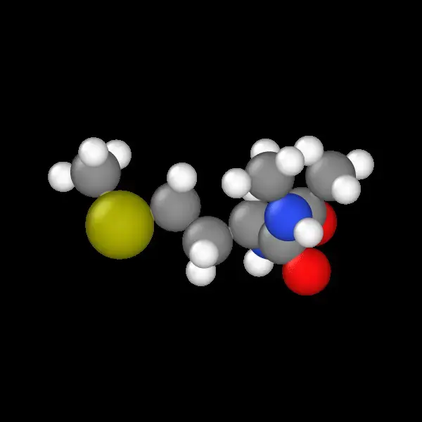
Special cases: Proline (ring constraint), Methionine (sulfur chemistry)

This systematic set allows studying how different chemical features affect dynamics:

• Does the flexibility of glycine lead to more diverse conformational sampling?
• How do aromatic rings in tryptophan affect folding pathways?
• Does the ring constraint in proline create different energy landscapes?

While these questions might seem basic, having systematic data to test ML models against known chemical intuition builds confidence in the approach.

Ideally, a neural network trained on this dataset should learn physical invariances. By training on both aliphatic (Val, Leu, Ile) and aromatic (Phe, Trp) systems, the model learns to distinguish how electron density (π-systems vs. σ-bonds) influences local potential energy surfaces, rather than just memorizing atom types.

Generating ML-Ready Trajectory Data

Generating raw coordinates is easy; generating ML-ready data requires specific configurations. Standard MD simulations compress trajectory files to save space, discarding high-frequency velocity and force data. To train Neural Network Potentials (NNPs), I configured the GROMACS pipeline differently.

The fastest way to generate trajectory data is using the run.sh script:

ID=ala ./scripts/run.sh

where ID is the three-letter amino acid code (here, ala for alanine).

This script performs energy minimization, solvation, neutralization, NVT equilibration, NPT equilibration, and production simulation. The resulting trajectory saves to the out/ID/data directory.

Why This Pipeline Differs from Standard Tutorials

A key deviation from standard tutorials is the use of Stochastic Dynamics (Langevin) as the integrator. This adds friction and noise terms to the equations of motion, ensuring correct thermodynamic sampling:

; config/md_langevin.mdp
integrator  = sd        ; Stochastic dynamics (Langevin)
dt          = 0.001     ; 1 fs timestep
nstxout     = 100       ; Save coordinates every 100 steps
nstvout     = 100       ; Save velocities every 100 steps
nstfout     = 100       ; Save forces every 100 steps
tc-grps     = Protein Non-Protein
tau_t       = 0.1  0.1  ; Friction constant (ps)
ref_t       = 298  298  ; Reference temperature (K)

The critical settings for ML applications:

1. Langevin Dynamics (sd): Ensures proper canonical (NVT) sampling rather than the deterministic velocity-rescaling often used in tutorials
2. Uncompressed Force Output (nstfout = 100): Writing to .trr format captures the precise atomic forces acting on every atom, essential for force-matching in NNP training
3. High-Frequency Sampling (0.1 ps): Saving frames every 100 fs captures fast bond vibrations often missed in standard 10 ps snapshots

Note: A production simulation currently runs for 1 nanosecond, saved every 0.1 picoseconds (100 fs). For most applications, increase this to 100 nanoseconds and adjust the save frequency to avoid large data files. I targeted 100 fs because I needed correlated time data for ML models, but you may not need such high frequency.

You can also run each step individually (see scripts/run.sh for examples).

The Systems

Here are the nine amino acid dipeptides I’ve included, each chosen for different chemical properties:

Alanine Dipeptide: The Standard

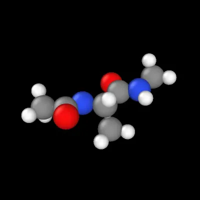
The classic starting point for protein folding studies. The small methyl side chain makes it simple but not trivial.

Glycine Dipeptide: Maximum Flexibility

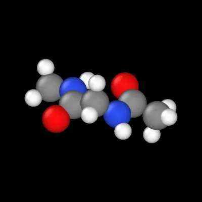
No side chain means maximum backbone flexibility. Great for studying how constraints affect conformational sampling.

Proline Dipeptide: Built-in Rigidity

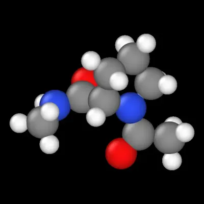
The ring structure creates backbone constraints. Interesting comparison to glycine’s flexibility.

Aromatic Systems

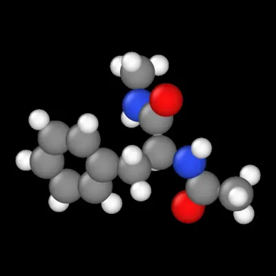
Phenylalanine: Simple benzene ring for studying aromatic interactions.

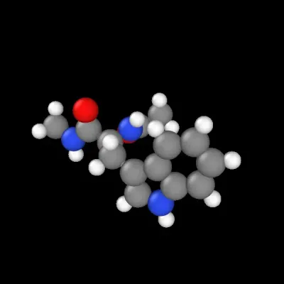
Tryptophan: Larger indole ring system with more complex aromatic chemistry.

Branched Aliphatic Systems

Valine: β-branched, creates steric constraints near the backbone.

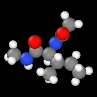
Isoleucine: γ-branched, different steric profile than valine.

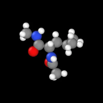
Leucine: Longer branched chain with more conformational freedom.

Special Chemistry

Methionine: Sulfur chemistry, different from the others and interesting for studying heteroatom effects.

What’s Next?

These mini-protein simulations have been useful for my ML work, providing systematic training data with controlled chemical variation. While they’re simple systems, they’ve helped me understand how different amino acid properties affect molecular behavior, knowledge that’s valuable when working with larger, more complex proteins.

The real value of this pipeline isn’t the simulations themselves, it’s the force extraction workflow. Having atomic forces alongside coordinates enables training NNPs via force matching, which typically converges faster and generalizes better than energy-only training. Tools like TorchMD-Net, NequIP, and MACE can directly consume this data format.

The scripts are designed to be easily modified for different amino acids or simulation conditions. I’ve tried to make the workflow straightforward while keeping it flexible.

This work complements my other molecular dynamics projects:

• Cu Adatom Diffusion: Learning LAMMPS for surface simulations
• Pt Adatom Diffusion: Extending to different elements

Together, these projects have given me a solid foundation in MD simulations for generating ML training data across different molecular systems.

Find the complete code and documentation on GitHub. Questions or suggestions? I’d love to hear from you, especially if you’ve found interesting ways to extend or improve the approach.

Acknowledgements

The scripts build on the GROMACS tutorial by Luca Tubiana at the University of Trento.