What is the Kabsch Algorithm?
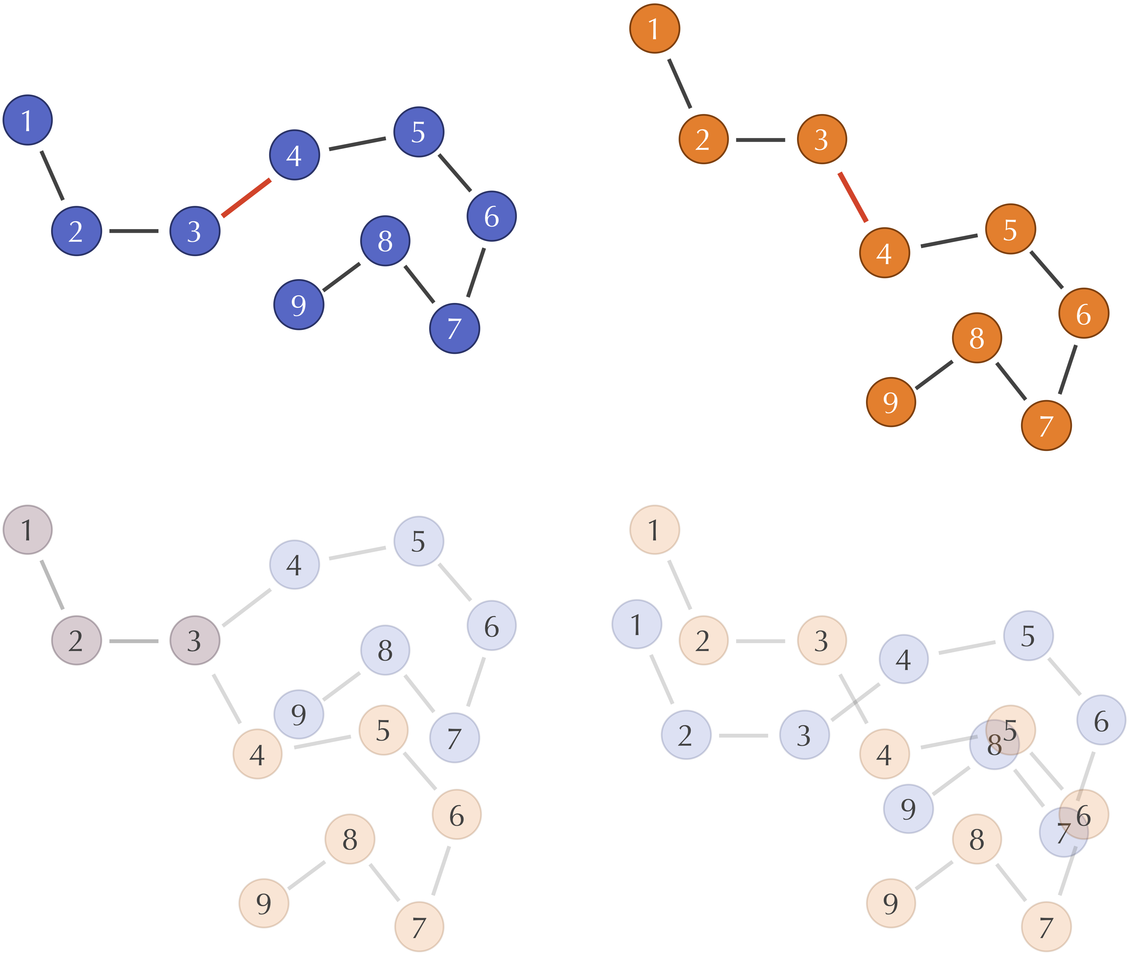
In computer vision or scientific computing, a common problem frequently arises: given two sets of points, what is the optimal rigid body transformation for their alignment? The Kabsch algorithm provides a nice solution.
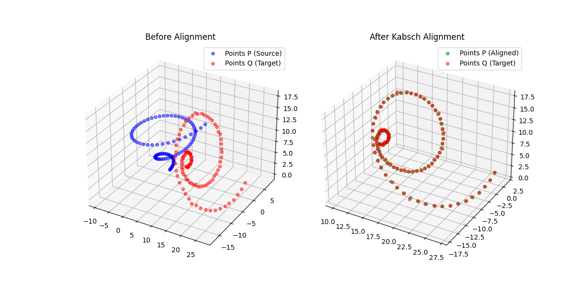
What are some concrete situations where this crops up?
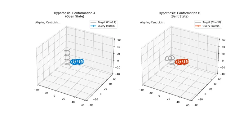
- Molecular Dynamics: Your points are a set of atoms (with physically relevant types), and you want to compare two molecular conformations. Are they the same structure with minor noise or rotation? Or are they different conformations, like a different folding of a protein? This is especially helpful when applying generative models to chemical structures. For example, if you are building a 3D Molecular VAE in PyTorch or working with Flow Matching models, Kabsch alignment ensures your generative loss function remains rotationally invariant.
- Computer Vision: You have two point clouds from 3D scans of an object taken from different angles. You want to align them to reconstruct the full shape. Or perhaps you’re generating 3D shapes from 2D images and need to compare the generated shape to a ground truth scan. Anytime a 3D system is represented as a point cloud, the Kabsch algorithm can help with alignment.
Of course, existing libraries implement this algorithm. However, often I find it beneficial to implement algorithms from scratch to build intuition. Furthermore, modern machine learning applications require automatic differentiation, so we will implement the algorithm in PyTorch, TensorFlow, and JAX.
Below, we’ll cover the math behind the Kabsch algorithm (and its scaling variant, the Kabsch-Umeyama algorithm) and provide complete, differentiable implementations in NumPy, PyTorch, TensorFlow, and JAX, demonstrating both single-pair and batched computations for ML applications.
The Math
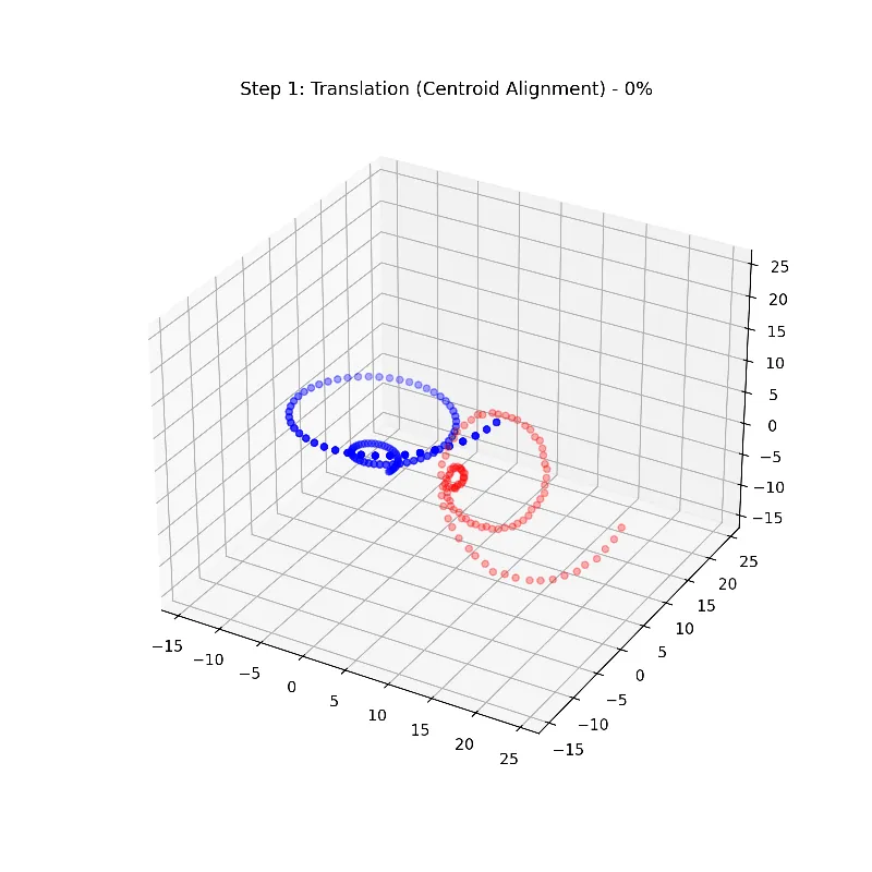
Let’s say we have two sets of paired points, $P={\mathbf{p}_i} \in \mathbb{R}^{N xD}$ and $Q={\mathbf{q}_i} \in \mathbb{R}^{N xD}$, for $i = 1, \dots, N$ (where $D$ is the dimensionality and $N$ is the number of points). We want to find a translation vector $\mathbf{t}$ and rotation matrix $R$ to transform $P$ to align with $Q$.
The optimization problem is:
$$ \min_{\mathbf{t}^\ast, \ R^\ast} \mathcal{L}(\mathbf{t}, R) = \frac{1}{2} \sum_{i=1}^N | \mathbf{q}_i - R(\mathbf{p}_i + \mathbf{t}) |^2 $$
where $\mathbf{t}^\ast \in \mathbb{R}^D$ and $R^\ast \in \mathbb{R}^{D xD}$ are the optimal translation and rotation.
Often we use a weighted version with weights $w_i$ (e.g., atomic masses in molecular dynamics):
$$ \min_{\mathbf{t}^\ast, \ R^\ast} \mathcal{L}(\mathbf{t}, R) = \frac{1}{2} \sum_{i=1}^N w_i | \mathbf{q}_i - R(\mathbf{p}_i + \mathbf{t}) |^2 $$
The Translation Vector
The translation vector is quite trivial to identify. Compute the centroids (averages) of both point sets:
$$ \bar{\mathbf{p}} = \frac{1}{N} \sum_{i=1}^N \mathbf{p_i} \quad \text{and}\ \bar{\mathbf{q}} = \frac{1}{N} \sum_{i=1}^N \mathbf{q}_i $$
Their optimal translation is their difference:
$$ \mathbf{t} = \bar{\mathbf{q}} - \bar{\mathbf{p}} $$
Specifically, the translation shifts the centroid of $P$ to the centroid of $Q$. After translation, we have:
$$ \mathbf{p}_i + \mathbf{t} = \bar{\mathbf{q}} + (\mathbf{p}_i - \bar{\mathbf{p}}) $$
and the remainder of their alignment reduces to finding the optimal rotation.
The Rotation Matrix
Computing the rotation matrix involves more calculation. First, center both point sets by subtracting their centroids:
$$ \mathbf{p}_i^\prime = \mathbf{p}_i - \bar{\mathbf{p}} \quad \text{and} \quad \mathbf{q}_i^\prime = \mathbf{q}_i - \bar{\mathbf{q}} $$
Next, compute the cross-covariance matrix between the centered sets:
$$ C = P^{\prime T} Q^\prime = \sum_{i=1}^N \mathbf{p}_i^{\prime T} \mathbf{q}_i^{\prime} \in \mathbb{R}^{D xD} $$
This is a fairly lightweight operation since $D$ is typically small (e.g., 3 for 3D points), even if $N$ is large.
With $C$ in hand, we want to compute its Singular Value Decomposition (SVD):
$$ C = U \Sigma V^T $$
This operation is computationally expensive. It scales cubically with $D$ (i.e., $O(D^3)$). However, since we’re often interested in cases where $D$ is small (e.g., 2D or 3D points), this is manageable.
Next, we check for improper rotations (i.e., reflections) and correct for them where necessary:
$$ d = \text{sign}(\det(V U^T)) $$
If $d = -1$, we need to flip the last column of $V$ in the final rotation matrix.
Let $B = \text{diag}(1, 1, d)$. The optimal rotation matrix comes out:
$$ R^\ast = V B U^T $$
Summary
In a nutshell, the Kabsch algorithm boils down to:
- Compute centroids of $P$ and $Q$ ($\bar{\mathbf{p}}$ and $\bar{\mathbf{q}}$)
- Center both point sets by subtracting centroids: $P^\prime$ and $Q^\prime$
- Compute cross-covariance matrix $C = P^{\prime T} Q^\prime$
- Compute SVD: $C = U \Sigma V^T$ (expensive step)
- Compute $d = \text{sign}(\det(V U^T))$ and $B = \text{diag}(1, 1, d)$
- Optimal rotation: $R^\ast = V B U^T$
- Optimal translation: $\mathbf{t}^\ast = \bar{\mathbf{q}} - \bar{\mathbf{p}}$
The resulting root-mean-square deviation (RMSD) between aligned point sets is
$$ \text{RMSD} = \sqrt{\frac{1}{N} \sum_{i=1}^N | \mathbf{q}_i - R^\ast(\mathbf{p}_i + \mathbf{t}^\ast) |^2} $$
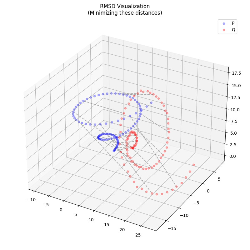
which is frequently used as a measure of similarity between molecular structures or as a metric in loss functions for ML applications.
The Kabsch-Umeyama Algorithm (Scaling)
While the standard Kabsch algorithm solves for optimal rotation and translation, the Kabsch-Umeyama algorithm extends this by also finding an optimal scaling factor $c$. This is essential when aligning structures of different scales, such as a 3D scan versus a ground truth model.
(Note: This is sometimes searched for as the “Absch-Umeyama algorithm” due to typos, but the correct attribution is to Shinji Umeyama based on Wolfgang Kabsch’s work.)
The method estimates the transformation $\mathbf{q}_i \approx c R \mathbf{p}_i + \mathbf{t}$. The optimal scale is given by the ratio of standard deviations of the point sets (after rotation).
A Note on SVD and Automatic Differentiation
While modern frameworks allow us to backpropagate through the Singular Value Decomposition (SVD), it comes with a known stability issue: if the cross-covariance matrix has identical (degenerate) singular values (which can occur if the point clouds are perfectly aligned or have certain symmetries), the gradient of the SVD approaches infinity, causing NaN values during backpropagation. If you plan to use this algorithm as a loss function for a neural network, it is often necessary to add a tiny epsilon to the matrix before computing the SVD, or to utilize an SVD gradient patch. The Kabsch-Horn Cookbook library provides a SafeSVD primitive that clamps the singular value gap in the backward pass, solving this problem across PyTorch, JAX, TensorFlow, and MLX.
Implementation
Let’s implement the algorithm in different frameworks. Note that for simplicity, the following implementations cover the unweighted Kabsch algorithm. If your application (like molecular dynamics) requires weights (e.g., atomic masses), the Kabsch-Horn Cookbook library provides per-point weighted alignment out of the box.
NumPy
import numpy as np


def kabsch_numpy(P, Q):
    """
    Computes the optimal rotation and translation to align two sets of points (P -> Q),
    and their RMSD.

    :param P: A Nx3 matrix of points
    :param Q: A Nx3 matrix of points
    :return: A tuple containing the optimal rotation matrix, the optimal
             translation vector, and the RMSD.
    """
    assert P.shape == Q.shape, "Matrix dimensions must match"

    # Compute centroids
    centroid_P = np.mean(P, axis=0)
    centroid_Q = np.mean(Q, axis=0)

    # Optimal translation
    t = centroid_Q - centroid_P

    # Center the points
    p = P - centroid_P
    q = Q - centroid_Q

    # Compute the covariance matrix
    H = np.dot(p.T, q)

    # SVD
    U, S, Vt = np.linalg.svd(H)

    # Validate right-handed coordinate system
    if np.linalg.det(np.dot(Vt.T, U.T)) < 0.0:
        Vt[-1, :] *= -1.0

    # Optimal rotation
    R = np.dot(Vt.T, U.T)

    # RMSD
    rmsd = np.sqrt(np.sum(np.square(np.dot(p, R.T) - q)) / P.shape[0])

    return R, t, rmsd
Here’s a quick test to verify correctness:
def test_numpy():
    np.random.seed(12345)

    P = np.random.randn(100, 3)

    alpha = np.random.rand() * 2 * np.pi
    R = np.array([[np.cos(alpha), -np.sin(alpha), 0],
                    [np.sin(alpha), np.cos(alpha), 0],
                    [0, 0, 1]])
    t = np.random.randn(3) * 10

    Q = np.dot(P, R.T) + t

    R_opt, t_opt, rmsd = kabsch_numpy(P, Q)

    print('RMSD: {}'.format(rmsd))
    print('R:\n{}'.format(R))
    print('R_opt:\n{}'.format(R_opt))
    print('t:\n{}'.format(t))
    print('t_opt:\n{}'.format(t_opt))

    l2_t = np.linalg.norm(t - t_opt)
    l2_R = np.linalg.norm(R - R_opt)
    print('l2_t: {}'.format(l2_t))
    print('l2_R: {}'.format(l2_R))
Running this test shows the algorithm correctly recovers the rotation and translation:
RMSD: 3.176703044042434e-15
R:
[[-0.8475392 -0.5307328  0.       ]
 [ 0.5307328 -0.8475392  0.       ]
 [ 0.         0.         1.       ]]
R_opt:
[[-8.47539198e-01 -5.30732803e-01 -8.26804079e-17]
 [ 5.30732803e-01 -8.47539198e-01 -8.32570352e-19]
 [ 8.20168388e-17  9.60990451e-18  1.00000000e+00]]
t:
[ 5.99726796  1.50078468 -3.34633977]
t_opt:
[ 6.10180512  1.50760274 -3.34633977]
l2_t: 0.10475926000353594
l2_R: 7.538724554724993e-16
The small differences are due to floating-point precision.
For batch processing:
def kabsch_numpy_batched(P, Q):
    """
    Computes the optimal rotation and translation to align two sets of points (P -> Q),
    and their RMSD.

    :param P: A BxNx3 matrix of points
    :param Q: A BxNx3 matrix of points
    :return: A tuple containing the optimal rotation matrix, the optimal
             translation vector, and the RMSD.
    """
    assert P.shape == Q.shape, "Matrix dimensions must match"

    # Compute centroids
    centroid_P = np.mean(P, axis=1, keepdims=True)  # Bx1x3
    centroid_Q = np.mean(Q, axis=1, keepdims=True)  # Bx1x3

    # Optimal translation
    t = centroid_Q - centroid_P  # Bx1x3
    t = t.squeeze(1)  # Bx3

    # Center the points
    p = P - centroid_P  # BxNx3
    q = Q - centroid_Q  # BxNx3

    # Compute the covariance matrix
    H = np.matmul(p.transpose(0, 2, 1), q)  # Bx3x3

    # SVD
    U, S, Vt = np.linalg.svd(H)  # Bx3x3

    # Validate right-handed coordinate system
    d = np.linalg.det(np.matmul(Vt.transpose(0, 2, 1), U.transpose(0, 2, 1)))
    flip = d < 0.0
    if flip.any():
        Vt[flip, -1, :] *= -1.0

    # Optimal rotation
    R = np.matmul(Vt.transpose(0, 2, 1), U.transpose(0, 2, 1))  # Bx3x3

    # RMSD
    rmsd = np.sqrt(np.sum(np.square(np.matmul(p, R.transpose(0, 2, 1)) - q), axis=(1, 2)) / P.shape[1])

    return R, t, rmsd
PyTorch
📝 Important Update (February 15, 2026)
Bug Fix Notice: The PyTorch implementation has been updated to use the “B-matrix” broadcasting approach. This eliminates in-place tensor modification (which breaks autograd) and data-dependent control flow (which breaks torch.compile and torch.vmap).
The PyTorch implementation now uses broadcasting to ensure differentiability:
import torch


def kabsch_torch(P, Q):
    """
    Computes the optimal rotation and translation to align two sets of points (P -> Q),
    and their RMSD.
    :param P: A Nx3 matrix of points
    :param Q: A Nx3 matrix of points
    :return: A tuple containing the optimal rotation matrix, the optimal
             translation vector, and the RMSD.
    """
    assert P.shape == Q.shape, "Matrix dimensions must match"

    # Compute centroids
    centroid_P = torch.mean(P, dim=0)
    centroid_Q = torch.mean(Q, dim=0)

    # Optimal translation
    t = centroid_Q - centroid_P

    # Center the points
    p = P - centroid_P
    q = Q - centroid_Q

    # Compute the covariance matrix
    H = torch.matmul(p.transpose(0, 1), q)

    # SVD
    U, S, Vt = torch.linalg.svd(H)

    # 1. Calculate determinant
    d = torch.det(torch.matmul(Vt.transpose(0, 1), U.transpose(0, 1)))

    # 2. Build diagonal B tensor without in-place mutation
    # We use stack to preserve gradients and graph connections
    B_diag = torch.stack([torch.tensor(1.0, device=d.device, dtype=d.dtype),
                          torch.tensor(1.0, device=d.device, dtype=d.dtype),
                          torch.sign(d)])

    # 3. Scale columns of Vt.T via broadcasting, then multiply by U^T
    # Vt.T: (3, 3). B_diag: (3) -> B_diag[None, :]: (1, 3)
    R = torch.matmul(Vt.transpose(0, 1) * B_diag[None, :], U.transpose(0, 1))

    # RMSD
    rmsd = torch.sqrt(torch.sum(torch.square(torch.matmul(p, R.transpose(0, 1)) - q)) / P.shape[0])

    return R, t, rmsd
And our batched version:
def kabsch_torch_batched(P, Q):
    """
    Computes the optimal rotation and translation to align two sets of points (P -> Q),
    and their RMSD, in a batched manner.
    :param P: A BxNx3 matrix of points
    :param Q: A BxNx3 matrix of points
    :return: A tuple containing the optimal rotation matrix, the optimal
             translation vector, and the RMSD.
    """
    assert P.shape == Q.shape, "Matrix dimensions must match"

    # Compute centroids
    centroid_P = torch.mean(P, dim=1, keepdims=True)  # Bx1x3
    centroid_Q = torch.mean(Q, dim=1, keepdims=True)  # Bx1x3

    # Optimal translation
    t = centroid_Q - centroid_P  # Bx1x3
    t = t.squeeze(1)  # Bx3

    # Center the points
    p = P - centroid_P  # BxNx3
    q = Q - centroid_Q  # BxNx3

    # Compute the covariance matrix
    H = torch.matmul(p.transpose(1, 2), q)  # Bx3x3

    # SVD
    U, S, Vt = torch.linalg.svd(H)  # Bx3x3

    # 1. Calculate batched determinant
    d = torch.det(torch.matmul(Vt.transpose(1, 2), U.transpose(1, 2)))  # B

    # 2. Build batched B_diag without in-place mutation or control flow
    ones = torch.ones_like(d)
    B_diag = torch.stack([ones, ones, torch.sign(d)], dim=-1) # Bx3

    # 3. Scale columns of Vt.T and multiply
    # Vt.T: (B, 3, 3). B_diag: (B, 3). B_diag[:, None, :]: (B, 1, 3).
    R = torch.matmul(Vt.transpose(1, 2) * B_diag[:, None, :], U.transpose(1, 2))

    # RMSD
    rmsd = torch.sqrt(torch.sum(torch.square(torch.matmul(p, R.transpose(1, 2)) - q), dim=(1, 2)) / P.shape[1])

    return R, t, rmsd
TensorFlow
The TensorFlow implementation returns S, U, and V directly. To handle immutability and potential compilation (e.g., via @tf.function), we avoid explicit conditional branching by constructing a correction matrix $B$ and broadcasting it.
import tensorflow as tf


def kabsch_tensorflow(P, Q):
    """
    Computes the optimal rotation and translation to align two sets of points (P -> Q),
    and their RMSD.

    :param P: A Nx3 matrix of points
    :param Q: A Nx3 matrix of points
    :return: A tuple containing the optimal rotation matrix, the optimal
             translation vector, and the RMSD.
    """
    P = tf.convert_to_tensor(P, dtype=tf.float32)
    Q = tf.convert_to_tensor(Q, dtype=tf.float32)

    assert P.shape == Q.shape, "Matrix dimensions must match"

    # Compute centroids
    centroid_P = tf.reduce_mean(P, axis=0)
    centroid_Q = tf.reduce_mean(Q, axis=0)

    # Optimal translation
    t = centroid_Q - centroid_P

    # Center the points
    p = P - centroid_P
    q = Q - centroid_Q

    # Compute the covariance matrix
    H = tf.matmul(tf.transpose(p), q)

    # SVD
    S, U, V = tf.linalg.svd(H)

    # 1. Calculate determinant
    # Note: V in TF SVD is V, not V^T.
    # R = V * U^T. Det(R) = Det(V * U^T)
    d = tf.linalg.det(tf.matmul(V, tf.transpose(U)))

    # 2. Build diagonal B tensor: [1.0, 1.0, sign(d)]
    # Use static shape 3 if possible, or infer from D. Assuming D=3 here.
    B_diag = tf.stack([1.0, 1.0, tf.sign(d)])

    # 3. Scale columns of V via broadcasting (V * B_diag), then multiply by U^T
    # V is DxD, B_diag is D. V * B_diag[None, :] multiplies each column j by B_diag[j]
    R = tf.matmul(V * B_diag[None, :], tf.transpose(U))

    # RMSD
    rmsd = tf.sqrt(tf.reduce_sum(tf.square(tf.matmul(p, tf.transpose(R)) - q)) / P.shape[0])

    return R, t, rmsd
and a batched version:
def kabsch_tensorflow_batched(P, Q):
    """
    Computes the optimal rotation and translation to align two sets of points (P -> Q),
    and their RMSD.

    :param P: A Nx3 matrix of points
    :param Q: A Nx3 matrix of points
    :return: A tuple containing the optimal rotation matrix, the optimal
             translation vector, and the RMSD.
    """
    P = tf.convert_to_tensor(P, dtype=tf.float32)
    Q = tf.convert_to_tensor(Q, dtype=tf.float32)

    assert P.shape == Q.shape, "Matrix dimensions must match"

    # Compute centroids
    centroid_P = tf.reduce_mean(P, axis=1, keepdims=True)
    centroid_Q = tf.reduce_mean(Q, axis=1, keepdims=True)

    # Optimal translation
    t = centroid_Q - centroid_P
    t = tf.squeeze(t, axis=1)

    # Center the points
    p = P - centroid_P
    q = Q - centroid_Q

    # Compute the covariance matrix
    H = tf.matmul(tf.transpose(p, perm=[0, 2, 1]), q)

    # SVD
    S, U, V = tf.linalg.svd(H)

    # 1. Calculate batched determinant
    d = tf.linalg.det(tf.matmul(V, tf.transpose(U, perm=[0, 2, 1])))

    # 2. Build batched B_diag: shape (B, 3)
    ones = tf.ones_like(d)
    B_diag = tf.stack([ones, ones, tf.sign(d)], axis=-1)

    # 3. Scale columns of V (Broadcasting adds the middle dimension)
    # V: (B, 3, 3), B_diag: (B, 3) -> B_diag[:, None, :]: (B, 1, 3)
    R = tf.matmul(V * B_diag[:, None, :], tf.transpose(U, perm=[0, 2, 1]))

    # RMSD
    rmsd = tf.sqrt(tf.reduce_sum(tf.square(tf.matmul(p, tf.transpose(R, perm=[0, 2, 1])) - q), axis=(1, 2)) / P.shape[1])

    return R, t, rmsd
JAX
The JAX implementation closely mirrors NumPy, replacing np with jnp. However, we again avoid if statements and in-place assignment (which JAX disallows) by using the broadcasting B-matrix approach.
import jax.numpy as jnp


def kabsch_jax(P, Q):
    """
    Computes the optimal rotation and translation to align two sets of points (P -> Q),
    and their RMSD.

    :param P: A Nx3 matrix of points
    :param Q: A Nx3 matrix of points
    :return: A tuple containing the optimal rotation matrix, the optimal
             translation vector, and the RMSD.
    """
    P = jnp.array(P)
    Q = jnp.array(Q)
    assert P.shape == Q.shape, "Matrix dimensions must match"

    # Compute centroids
    centroid_P = jnp.mean(P, axis=0)
    centroid_Q = jnp.mean(Q, axis=0)

    # Optimal translation
    t = centroid_Q - centroid_P

    # Center the points
    p = P - centroid_P
    q = Q - centroid_Q

    # Compute the covariance matrix
    H = jnp.dot(p.T, q)

    # SVD
    U, S, Vt = jnp.linalg.svd(H)

    # 1. Calculate determinant
    d = jnp.linalg.det(jnp.dot(Vt.T, U.T))

    # 2. Build diagonal B array
    B_diag = jnp.array([1.0, 1.0, jnp.sign(d)])

    # 3. Scale columns of Vt.T and multiply by U.T
    # Vt.T is V.
    R = jnp.dot(Vt.T * B_diag[None, :], U.T)

    # RMSD
    rmsd = jnp.sqrt(jnp.sum(jnp.square(jnp.dot(p, R.T) - q)) / P.shape[0])

    return R, t, rmsd
and batched:
def kabsch_jax_batched(P, Q):
    """
    Computes the optimal rotation and translation to align two sets of points (P -> Q),
    and their RMSD.

    :param P: A BxNx3 matrix of points
    :param Q: A BxNx3 matrix of points
    :return: A tuple containing the optimal rotation matrix, the optimal
             translation vector, and the RMSD.
    """
    P = jnp.array(P)
    Q = jnp.array(Q)
    assert P.shape == Q.shape, "Matrix dimensions must match"

    # Compute centroids
    centroid_P = jnp.mean(P, axis=1, keepdims=True)  # Bx1x3
    centroid_Q = jnp.mean(Q, axis=1, keepdims=True)  # Bx1x3

    # Optimal translation
    t = centroid_Q - centroid_P  # Bx1x3
    t = t.squeeze(1)  # Bx3

    # Center the points
    p = P - centroid_P  # BxNx3
    q = Q - centroid_Q  # BxNx3

    # Compute the covariance matrix
    H = jnp.matmul(p.transpose(0, 2, 1), q)  # Bx3x3

    # SVD
    U, S, Vt = jnp.linalg.svd(H)  # Bx3x3

    # 1. Calculate batched determinant
    d = jnp.linalg.det(jnp.matmul(Vt.transpose(0, 2, 1), U.transpose(0, 2, 1)))

    # 2. Build batched B_diag
    ones = jnp.ones_like(d)
    B_diag = jnp.stack([ones, ones, jnp.sign(d)], axis=-1)

    # 3. Scale columns of Vt.T and multiply by U.T
    # Vt.T: (B, 3, 3). B_diag: (B, 3).
    R = jnp.matmul(Vt.transpose(0, 2, 1) * B_diag[:, None, :], U.transpose(0, 2, 1))

    # RMSD
    rmsd = jnp.sqrt(jnp.sum(jnp.square(jnp.matmul(p, R.transpose(0, 2, 1)) - q), axis=(1, 2)) / P.shape[1])

    return R, t, rmsd
Extensions
The Kabsch algorithm has several important extensions that go beyond the formulation dealt with here:
- Quaternion Form: The algorithm can be reformulated using quaternions for better numerical stability, particularly useful in applications requiring high precision.
- Iterative Versions: More robust variants that handle noise better and have improved scaling properties for large point sets. This also can be advantageous for setups with limited computational resources.
- Weighted Kabsch: Extensions that incorporate point weights (e.g., atomic masses in molecular dynamics). While SciPy provides a weighted version, it lacks batch processing capabilities.
- The Umeyama Algorithm: If your point sets are rotated, translated, and scaled differently, the Umeyama algorithm is the direct extension of Kabsch. It solves the same optimization problem but introduces a scaling factor $c$, finding the optimal alignment for $Q \approx c R P + t$.
Several of these extensions are implemented in the Kabsch-Horn Cookbook library, which provides differentiable Kabsch, Horn, and Umeyama alignment across NumPy, PyTorch, JAX, TensorFlow, and MLX.
Further Reading
- Wikipedia, Kabsch Algorithm
- Zalo on Kabsch: An interactive shape matching demo.
Original Papers
- [Kabsch 1976] Kabsch, W. (1976). “A solution for the best rotation to relate two sets of vectors.” Acta Crystallographica Section A, 32(5), 922-923. DOI: 10.1107/S0567739476001873 The original paper introducing the SVD-based alignment. See also: paper notes.
- [Kabsch 1978] Kabsch, W. (1978). “A discussion of the solution for the best rotation to relate two sets of vectors.” Acta Crystallographica Section A, 34(5), 827-828. DOI: 10.1107/S0567739478001680 The follow-up paper correcting for improper rotations (reflections).
- [Arun et al. 1987] Arun, K. S., Huang, T. S., & Blostein, S. D. (1987). “Least-Squares Fitting of Two 3-D Point Sets.” IEEE Transactions on Pattern Analysis and Machine Intelligence, PAMI-9(5), 698-700. DOI: 10.1109/TPAMI.1987.4767965 The first SVD-based formulation for 3D point set alignment. See also: paper notes.
- [Horn et al. 1988] Horn, B. K. P., Hilden, H. M., & Negahdaripour, S. (1988). “Closed-form solution of absolute orientation using orthonormal matrices.” Journal of the Optical Society of America A, 5(7), 1127-1135. DOI: 10.1364/JOSAA.5.001127 The matrix square root (polar decomposition) approach to the same problem. See also: paper notes.
- [Horn 1987] Horn, B. K. P. (1987). “Closed-form solution of absolute orientation using unit quaternions.” Journal of the Optical Society of America A, 4(4), 629-642. DOI: 10.1364/JOSAA.4.000629 An alternative quaternion-based closed-form solution that also handles scale. See also: paper notes.
- [Umeyama 1991] Umeyama, S. (1991). “Least-squares estimation of transformation parameters between two point patterns.” IEEE Transactions on Pattern Analysis and Machine Intelligence, 13(4), 376-380. DOI: 10.1109/34.88573 The extension of the algorithm to include optimal scaling in addition to rotation and translation. See also: paper notes.
