Word Embeddings in NLP: An Introduction

Understanding Word Embeddings

A word embedding maps words to real-valued vectors:

$$ \text{word} \rightarrow \mathbb{R}^n $$

where $n$ represents the dimensionality of the embedding space.

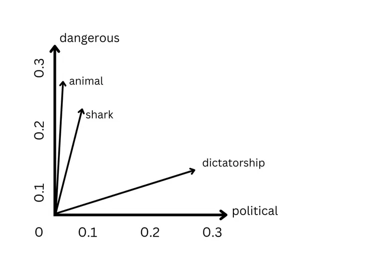
The goal is simple: position semantically similar words close together in vector space. This dense representation typically uses hundreds of dimensions, a massive reduction from the millions required by one-hot encoding.

Word embeddings are grounded in Zellig Harris’ distributional hypothesis: words appearing in similar contexts tend to have similar meanings. This forms the foundation of distributional semantics.

Different embedding algorithms capture various aspects of this distributional principle. This post explores the main methods for creating word embeddings and their applications in natural language processing.

While modern foundation models and terabyte-scale Vision-Language Models (VLMs) rely on advanced subword tokenizers (like BPE) and massive Transformer embedding layers, the fundamental goal remains exactly the same: mapping discrete text to a continuous vector space where math can capture meaning. Understanding these foundational techniques provides the necessary intuition for debugging and scaling today’s production ML systems.

Why Word Embeddings Matter in NLP

Computers require numerical representations to apply machine learning algorithms to text. Word embeddings bridge this gap by converting text into dense vectors that preserve semantic and syntactic relationships.

Key advantages:

1. Dense representation: Hundreds of dimensions provide a compact alternative to vocabulary-sized sparse vectors.
2. Semantic preservation: Similar words cluster together in vector space.
3. Mathematical operations: Enable analogical reasoning ($\text{king} - \text{man} + \text{woman} \approx \text{queen}$).
4. Transfer learning: Pre-trained embeddings work across multiple tasks and domains.

Modern deep learning architectures leverage these properties extensively. The development of universal, pre-trained embeddings was a significant step forward. We can use versatile embeddings that generalize across applications, eliminating the need to train task-specific representations from scratch.

Word Embedding Approaches

One-Hot Encoding and Count Vectorization

One-hot encoding represents the simplest approach to word vectorization. Each word gets a unique dimension in a vocabulary-sized vector, marked with 1 for presence and 0 elsewhere. Count vectorization extends this by counting the occurrences of each word in a document.

Characteristics:

• High dimensionality: Vector length equals vocabulary size.
• Extreme sparsity: Most dimensions contain zeros.
• No relationships: Treats all words as equally distant.
• Computational efficiency: Simple to implement and understand.

While lacking semantic information, count vectorization serves as a foundation for more complex methods. Let’s look at a practical implementation using scikit-learn’s CountVectorizer.

from sklearn.feature_extraction.text import CountVectorizer

# Initialize the vectorizer
vectorizer = CountVectorizer()

# Sample text for demonstration
sample_text = ["One of the most basic ways we can numerically represent words "
               "is through the one-hot encoding method (also sometimes called "
               "count vectorizing)."]

# Fit the vectorizer to our text data
vectorizer.fit(sample_text)

# Examine the vocabulary and word indices
print('Vocabulary:')
print(vectorizer.vocabulary_)

# Transform text to vectors
vector = vectorizer.transform(sample_text)
print('Full vector:')
print(vector.toarray())

In a production environment, count vectorization introduces significant engineering challenges. When processing millions of documents, the vocabulary size explodes. Storing and computing on these massive sparse matrices quickly leads to memory exhaustion. In these scaling scenarios, practitioners often turn to the Hashing Trick (via HashingVectorizer) to bound the dimensionality, or they move entirely to the dense embeddings discussed later in this post.

We can see count vectorization in action with a real dataset, building a simple text classifier for the 20 Newsgroups dataset:

from sklearn.datasets import fetch_20newsgroups
from sklearn.feature_extraction.text import CountVectorizer
from sklearn.naive_bayes import MultinomialNB
from sklearn import metrics

# Load train and test splits, removing metadata for a cleaner signal
newsgroups_train = fetch_20newsgroups(subset='train',
                                      remove=('headers', 'footers', 'quotes'))
newsgroups_test = fetch_20newsgroups(subset='test',
                                     remove=('headers', 'footers', 'quotes'))

# Initialize and fit vectorizer on training data
vectorizer = CountVectorizer()
X_train = vectorizer.fit_transform(newsgroups_train.data)

# Build and train classifier
classifier = MultinomialNB(alpha=0.01)
classifier.fit(X_train, newsgroups_train.target)

# Transform test data and make predictions
X_test = vectorizer.transform(newsgroups_test.data)
y_pred = classifier.predict(X_test)

# Evaluate performance
accuracy = metrics.accuracy_score(newsgroups_test.target, y_pred)
print(f'Accuracy: {accuracy:.3f}')

This provides a solid baseline. To capture actual semantic meaning and reduce dimensionality, we must move beyond simple counting.

TF-IDF (Term Frequency-Inverse Document Frequency)

TF-IDF extends one-hot encoding by weighting terms based on their importance across a document collection. TF-IDF combines:

• Term Frequency (TF): How often a word appears in a document
• Inverse Document Frequency (IDF): How rare a word is across all documents

This weighting scheme reduces the impact of common words (like “the” or “and”) while emphasizing distinctive terms that appear frequently in specific documents but rarely elsewhere.

Advantages:

• Captures document-level importance
• Reduces impact of stop words
• Effective for information retrieval tasks

Limitations:

• Still high-dimensional and sparse
• No semantic relationships between terms
• Context-independent representation

Co-Occurrence Matrices

Co-occurrence matrices capture word relationships by recording which terms appear together within defined contexts (sentences, paragraphs, or fixed windows). The resulting matrix has dimensions equal to vocabulary size squared, with entries showing co-occurrence frequency.

Key properties:

• Global statistics: Captures corpus-wide word relationships
• Symmetric relationships: Mutual co-occurrence patterns
• Extreme dimensionality: Vocabulary size squared creates storage challenges
• Sparse representation: Most word pairs never co-occur

While computationally expensive to store and process, co-occurrence matrices form the foundation for advanced methods like GloVe that compress this information into dense representations.

Neural Network-Based Embeddings

Neural Probabilistic Language Models

Neural probabilistic models pioneered the use of neural networks for learning word embeddings. These models learn dense representations as a byproduct of language modeling, predicting the next word in a sequence.

Training process:

1. Initialize random dense embeddings for each vocabulary word
2. Use embeddings as inputs to predict language modeling objectives
3. Update embeddings through backpropagation based on prediction errors
4. Resulting embeddings capture patterns useful for the training task

This approach demonstrated that task-specific embeddings could be learned jointly with model objectives, establishing the foundation for modern embedding methods.

Word2Vec

Word2Vec revolutionized word embeddings by introducing efficient training algorithms for massive corpora. It became the first method to demonstrate compelling vector arithmetic properties, enabling analogical reasoning like the famous “$\text{king} - \text{man} + \text{woman} \approx \text{queen}$” example.

Two training architectures:

Continuous Bag-of-Words (CBOW)

Predicts target words from surrounding context words. Given a window of context words, the model learns to predict the central word.

Skip-Gram

Predicts context words from target words. Given a central word, the model learns to predict surrounding words within a defined window.

Key advantages:

• Computational efficiency: Much faster than neural probabilistic models
• Scalable training: Can process billion-word corpora effectively
• Quality embeddings: Captures semantic and syntactic relationships
• Flexible context: Window size controls topical vs. functional similarity

The choice of window size significantly impacts learned relationships. Larger windows capture topical associations, while smaller windows focus on syntactic and functional similarities.

GloVe (Global Vectors)

GloVe combines the best aspects of matrix factorization methods (which capture global corpus statistics) and local context window approaches like Word2Vec. Matrix factorization methods excel at global patterns but struggle with analogical reasoning, while Word2Vec captures local relationships but may miss global structure.

Key innovation: GloVe trains on a global word-context co-occurrence matrix, incorporating corpus-wide statistical information while maintaining the analogical reasoning capabilities that made Word2Vec successful.

Advantages over Word2Vec:

• Global optimization: Leverages entire corpus statistics
• Better performance: Often outperforms Word2Vec on word similarity and analogy tasks
• Stable training: More consistent convergence due to global objective function

The result is embeddings that capture both local syntactic patterns and global semantic relationships more effectively.

Contextual Embedding Methods

FastText

FastText addresses a critical limitation of previous methods: handling out-of-vocabulary (OOV) words. By incorporating subword information, FastText can generate meaningful representations for previously unseen words.

Subword approach:

• Decomposes words into character n-grams (typically 3-6 characters)
• Represents words as sums of their component n-grams
• Trains using skip-gram objective with negative sampling

Key advantages:

• OOV handling: Can embed unseen words using known subword components
• Morphological awareness: Captures relationships between related word forms
• Multilingual support: Facebook released pre-trained embeddings for 294 languages
• Robust performance: Particularly effective for morphologically rich languages

For example, if the model knows “navigate,” it can provide meaningful representation for “circumnavigate” by leveraging shared subword components, even if “circumnavigate” wasn’t in the training data.

Poincaré Embeddings

Poincaré embeddings introduce a novel approach by learning representations in hyperbolic space. This geometric innovation specifically targets hierarchical relationships in data.

Hyperbolic geometry advantages:

• Natural hierarchy encoding: Distance represents similarity, while norm encodes hierarchical level
• Efficient representation: Requires fewer dimensions for hierarchical data
• Mathematical elegance: Leverages properties of hyperbolic space for embedding optimization

Applications: Particularly effective for data with inherent hierarchical structure, such as:

• WordNet taxonomies
• Organizational charts
• Computer network topologies
• Knowledge graphs

The original paper demonstrates good efficiency in reproducing WordNet relationships with significantly lower dimensionality compared to traditional embedding methods.

Contextual Embeddings

ELMo (Embeddings from Language Models)

ELMo represents a paradigm shift toward contextual word representations. ELMo generates dynamic representations based on sentence context, adapting to word usage patterns.

Architecture:

• Bidirectional LSTM: Processes text in both forward and backward directions
• Character-level input: Handles OOV words and captures morphological patterns
• Multi-layer representations: Combines different abstraction levels

Layer specialization:

• Lower layers: Excel at syntactic tasks (POS tagging, parsing)
• Higher layers: Capture semantic relationships (word sense disambiguation)
• Combined layers: Weighted combination achieves good performance

Key innovation: ELMo embeddings vary by context. The word “bank” receives different representations in “river bank” versus “financial bank,” addressing polysemy directly through contextual awareness.

This approach achieved strong performance across numerous NLP tasks by providing context-sensitive representations that adapt to word usage patterns.

Probabilistic FastText

Probabilistic FastText addresses polysemy (words with multiple meanings) through probabilistic modeling. Traditional embeddings conflate different word senses into single representations, limiting their precision.

The polysemy problem: Consider “rock” which can mean:

• Rock music (genre)
• A stone (geological object)
• Rocking motion (verb)

Standard embeddings average these meanings, producing representations that may not capture any sense precisely.

Probabilistic approach: Probabilistic FastText represents words as Gaussian mixture models: probability distributions that can capture multiple distinct meanings as separate components.

Advantages:

• Multi-sense representation: Each word sense gets its own distribution
• Context sensitivity: Can select appropriate sense based on usage context
• Uncertainty quantification: Probabilistic framework captures embedding confidence

This approach provides a more nuanced treatment of lexical ambiguity, particularly valuable for words with distinct, context-dependent meanings.

Summary and Future Directions

Word embeddings have evolved from simple one-hot encodings to contextual representations that capture nuanced linguistic relationships. Each approach offers distinct advantages:

Static embeddings (Word2Vec, GloVe, FastText) provide:

• Computational efficiency for large-scale applications
• Pre-trained models available for numerous languages
• Clear analogical reasoning capabilities
• Good performance on many downstream tasks

Contextual embeddings (ELMo, BERT, GPT) offer:

• Dynamic representations based on sentence context
• Better handling of polysemy and word sense disambiguation
• Strong performance on complex NLP tasks
• Ability to capture subtle contextual nuances

Choosing the right approach depends on:

• Task requirements: Static embeddings for efficiency, contextual for accuracy
• Data availability: Pre-trained models vs. domain-specific training
• Computational constraints: Static embeddings require less processing power
• Language coverage: Consider availability of pre-trained models for target languages

The field continues advancing toward more efficient contextual models, better multilingual representations, and embeddings that capture increasingly complex linguistic phenomena.