GEOM Dataset: 3D Molecular Conformer Generation

Introduction

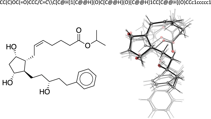
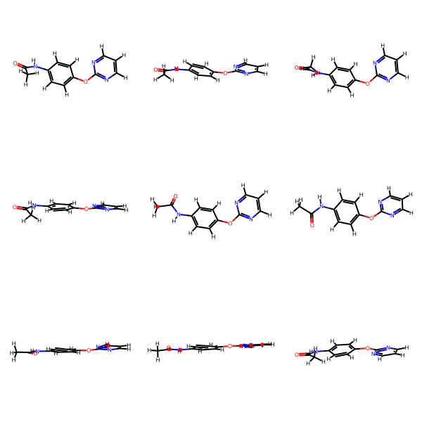
In molecular machine learning, we often start with a 2D graph—a blueprint of atoms and bonds. But this blueprint misses a crucial detail: a molecule’s function is deeply tied to its dynamic 3D shape. In reality, a molecule isn’t static; it’s a flexible entity that exists as an ensemble of low-energy conformations. Capturing 3D molecular shapes is crucial for predicting molecular behavior.

The GEOM (Geometric Ensemble Of Molecules) dataset was created to bridge this gap. It provides a massive collection of high-quality 3D conformer ensembles, transforming static 2D graphs into something much closer to physical reality. This makes it an invaluable resource for anyone working in geometric deep learning for chemistry and drug discovery.

The Challenge of Conformer Generation

So, why don’t we just generate 3D structures for every molecule? It’s computationally hard for two main reasons:

1. Combinatorial Explosion: Think of a molecule with several rotatable bonds. Each bond is like a joint that can be twisted. The number of possible 3D shapes grows exponentially with each new joint. Trying every combination is impractical for most molecules.
2. Speed vs. Accuracy: We need to calculate the energy of each shape to know if it’s realistic (low energy) or not (high energy). Classical force fields are fast but often inaccurate. On the other end, Density Functional Theory (DFT) provides quantum mechanical accuracy but is far too slow to generate millions of conformations needed for a large dataset.

GEOM strikes a balance by using a semi-empirical method that’s much faster than DFT but still captures the underlying quantum mechanics far better than classical force fields.

A Deeper Look Inside the GEOM Dataset

The scale of GEOM is impressive: over 37 million conformations for more than 450,000 unique molecules. But the numbers in the paper’s tables tell a more interesting story about the dataset’s composition.

A simplified view of Tables 1 & 4 from the paper, highlighting the key differences.

What does this tell us?

• Two Worlds of Molecules: The dataset is clearly split. The QM9 subset contains small, relatively rigid molecules (mean of 2.2 rotatable bonds). In contrast, the AICures subset contains larger, more flexible drug-like molecules (mean of 6.5 rotatable bonds, with one molecule having 53!). This diversity is ideal for training machine learning models that need to generalize from simple cases to complex, real-world examples.
• Conformational Complexity: The number of conformers found per molecule reflects this flexibility. A typical QM9 molecule has about 13 conformers, while a drug-like molecule has over 100 on average. This highlights why a single 3D structure is often not enough for flexible molecules.

Beyond the structures themselves, GEOM is rich with experimental data, connecting the 3D shapes to real-world properties. The molecules are labeled with data for everything from water solubility and blood-brain barrier penetration to toxicity and inhibition of key viral targets like the SARS-CoV-2 3CL protease. This makes it a powerful tool for developing property prediction models.

In fact, this creates a benchmark for:

• Property prediction models that can leverage conformer ensembles (or members of the ensemble) as input.
• Conformer generation models that must transform 2D graphs into realistic, 3D distributions.
• End-to-end property-based evaluation of the conformer ensembles generated by a model.

The Toolbox Behind GEOM: Key Techniques Explained

The GEOM paper mentions several advanced computational chemistry methods. Let’s briefly break down the most important ones:

• GFN2-xTB: This is the semi-empirical quantum mechanical method used to calculate energies and forces in GEOM. Think of it as a “middle ground” method. It’s much faster than full DFT but captures electronic effects that classical force fields miss, making it a pragmatic choice for generating a large dataset.
• CREST: This is the program that actually performs the conformer search. It uses a clever technique based on metadynamics, where it simulates the molecule’s movement and adds a “penalty” potential to discourage it from revisiting shapes it has already seen. This pushes the molecule to explore its conformational space efficiently, finding many diverse, low-energy structures.
• CENSO: For a small subset of molecules, the authors went a step further with CENSO. This program takes the conformers found by CREST and refines them with more accurate (and expensive) DFT calculations. It’s a way of getting very high-quality “gold standard” data for benchmarking.
• Implicit Solvent Models: Molecules in the body are rarely in a vacuum; they’re usually in water. Methods like C-PCM and ALPB model water as a continuous medium, which affects the molecule’s preferred shape and energy. This is crucial for biological applications.

The Math Behind the Molecules (Explained Simply)

The paper includes a couple of equations based on the Boltzmann distribution, which is a fundamental concept from statistical mechanics that tells us the probability of finding a system in a certain state.

The key equation used by CREST to assign a probability (or “statistical weight”) to the i-th conformer is:

$$ P*{i}^{\text{CREST}} = \frac{d*{i}\exp(-E*{i}/k*{B}T)}{\sum*{j}d*{j}\exp(-E*{j}/k*{B}T)} $$

Let’s demystify this:

• $E_i$ is the energy of the conformer. The negative sign and the exponential mean that lower energy leads to a much higher probability.
• $k_B T$ is the thermal energy at a given temperature $T$. It sets the energy scale. If the energy difference between two conformers is much larger than $k_B T$, the higher-energy one will be virtually nonexistent.
• $d_i$ represents the degeneracy of the conformer, which accounts for the number of equivalent states or configurations that share the same energy $E_i$.
  • Degeneracy refers to the number of equivalent, indistinguishable atomic arrangements (rotamers) that correspond to a single overall molecular shape (conformer). For example, the rotation of a methyl group (–CH₃) produces multiple identical-looking orientations of its hydrogen atoms.
• The denominator, $\sum_{j}d_{j}\exp(-E_{j}/k_{B}T)$, is the partition function. Its job is to sum up the terms from all possible conformers to ensure that all the probabilities add up to 100%.

For the high-quality CENSO calculations, the equation is similar but uses the Gibbs Free Energy ($G_i$) instead of the potential energy ($E_i$). Free energy is a more complete measure because it includes not just the molecule’s internal energy, but also its interaction with a solvent and entropic effects (like how much it can “wiggle”). This gives a more accurate ranking of the conformer probabilities.

A Closer Look at the Figures: What the Data Really Shows

The paper’s figures offer some honest insights into the dataset’s quality and the trade-offs involved.

Figure 3 is particularly important. It compares the fast GFN2-xTB energies with much more accurate single-point DFT energies.

• The Mean Absolute Error (MAE) of 1.96 kcal/mol shows that, on average, the fast method gets the energy wrong by about 2 kcal/mol. At room temperature, the thermal energy ($k_B T$) is only about 0.6 kcal/mol. Because the Boltzmann probability depends on the energy exponentially, a 2 kcal/mol error can dramatically change the predicted importance of a conformer.
• The Spearman correlation plot (right side) shows how well GFN2-xTB ranks the conformers from lowest to highest energy compared to DFT. An average correlation of 0.39 is okay—it’s much better than random—but the distribution is very wide. For some molecules, the ranking is nearly perfect, while for others it’s quite poor.

This is a key takeaway: the GFN2-xTB/CREST method is excellent for discovering the right set of low-energy shapes, but not as reliable for ranking them by probability. For accurate ranking, the higher-level DFT energies also provided in GEOM are the way to go.

Conclusion: What This Means for Machine Learning

For researchers at the intersection of machine learning and chemistry, GEOM provides more than just data; it provides a realistic foundation to build upon. By shifting the focus from static 2D graphs to dynamic 3D ensembles, GEOM enables a new generation of models.

This dataset is an ideal training ground for models designed to understand 3D geometry, such as SE(3)-equivariant neural networks and diffusion models, which can learn to generate conformer ensembles directly from a 2D graph. By training on GEOM, these models can learn the complex relationship between a molecule’s chemical blueprint and its real-world, flexible nature.

For a comprehensive technical reference including detailed specifications, quality metrics, and performance leaderboards, see my GEOM Dataset Card.

Explore the GEOM dataset further by visiting its GitHub repository.

References

• Axelrod, S. & Gómez-Bombarelli, R. “GEOM, energy-annotated molecular conformations for property prediction and molecular generation.” Scientific Data 9, 185 (2022). https://doi.org/10.1038/s41597-022-01288-4
• GitHub repositories:
  • learningmatter-mit/geom
  • learningmatter-mit/NeuralForceField