Classifying Congressional Bills with Machine Learning

Introduction

This post explores machine learning approaches for classifying congressional bills by policy area, using data from the 115th to 117th Congresses (2017-2023). We’ll examine:

The fundamentals of bill classification
Traditional machine learning models as baselines
Performance analysis across different time periods and policy domains

This work establishes baselines for future deep learning approaches to legislative text classification.

This post builds on the data foundation established in Exploring the 117th U.S. Congress.

Why This Matters

Automatically classifying congressional bills by policy area has practical value for researchers, journalists, and citizens who need to navigate thousands of bills each Congress. Machine learning can help identify patterns in legislative priorities and track policy trends over time.

This work establishes baseline performance for text classification on legislative data, providing a foundation for more sophisticated approaches.

Data

The data comes from scraping Congress.gov for all bills from the 115th through 117th Congresses. Each bill includes:

Bill ID and title
Summary (when available) - the earliest summary provided
Full text (when available) - the earliest text version
Policy area classification

Our task is to predict policy area from text features:

$$ f(X) = \hat{y}, \quad \text{where} \quad X = { \text{title}, \text{summary}, \text{text} }, \quad \hat{y} \in { \text{policy areas} } $$

The complete dataset is available at Hugging Face: hheiden/us-congress-bill-policy-115_117.

Bills by Congress

Our dataset contains the following distribution:

Congress	Bills
115th	13,555
116th	16,601
117th	17,817
Total	47,973

Policy Areas

Each bill receives a policy area label from Congress.gov (see glossary). The dataset includes 33 policy areas, though these classes are highly imbalanced.

The following table shows the number of bills in each policy area across the three Congresses:

Policy Area	115th	116th	117th	Total
Agriculture and Food	312	328	398	1,038
Animals	96	83	71	250
Armed Forces and National Security	1,108	1,337	1,399	3,844
Arts, Culture, Religion	81	79	103	263
Civil Rights and Liberties, Minority Issues	175	205	220	600
Commerce	312	593	633	1,538
Congress	594	541	640	1,775
Crime and Law Enforcement	827	904	1,022	2,753
Economics and Public Finance	176	210	197	583
Education	607	798	801	2,206
Emergency Management	207	198	202	607
Energy	316	370	530	1,216
Environmental Protection	352	423	464	1,239
Families	79	127	139	345
Finance and Financial Sector	556	611	601	1,768
Foreign Trade and International Finance	120	148	212	480
Government Operations and Politics	1,008	1,258	1,272	3,538
Health	1,526	2,109	2,276	5,911
Housing and Community Development	142	250	231	623
Immigration	398	466	591	1,455
International Affairs	918	1,178	1,390	3,486
Labor and Employment	348	452	552	1,352
Law	109	162	175	446
Native Americans	175	234	245	654
Public Lands and Natural Resources	718	648	642	2,008
Science, Technology, Communications	389	551	505	1,445
Social Sciences and History	5	6	4	15
Social Welfare	177	229	199	605
Sports and Recreation	92	93	125	310
Taxation	983	1,156	1,078	3,217
Transportation and Public Works	492	672	742	1,906
Water Resources Development	89	111	110	310
Private Legislation	69	71	48	188

The class imbalance is severe: Social Sciences and History has only 15 bills across all three Congresses, while Health has 5,911 bills. This imbalance presents modeling challenges, as minority classes may lack sufficient representative samples.

Text Statistics

We analyzed token counts using spaCy to understand the computational requirements for each text field.

Title Token Statistics:

Congress	Average Tokens	Min Tokens	Max Tokens	Total Tokens
115th	12.3	1	167	166,763
116th	11.3	1	226	188,158
117th	11.5	1	272	204,978
All	11.7	1	272	559,419

Summary Token Statistics:

Congress	Average Tokens	Min Tokens	Max Tokens	Total Tokens
115th	109.1	2	6,839	1,479,212
116th	94.9	2	5,886	1,574,732
117th	95.1	2	502	1,695,276
All	99.0	2	6,839	4,749,220

Full Text Token Statistics:

Congress	Average Tokens	Min Tokens	Max Tokens	Total Tokens
115th	2,588.7	91	304,478	35,092,075
116th	2,760.3	70	973,173	45,824,498
117th	2,706.7	71	1,013,608	48,224,757
All	-	70	1,013,608	129,141,330

These statistics reveal computational trade-offs:

Titles average ~12 tokens - computationally efficient but limited information
Summaries average ~100 tokens - good balance of information and efficiency
Full text averages ~2,700 tokens with 129M total tokens - detailed but computationally expensive

We’ll prototype with titles and summaries before considering full text, given the computational costs involved.

Evaluation Framework

Experimental Design

We train models on one Congress and test on others, creating a 3×3 evaluation grid. This setup evaluates both within-Congress performance (same session) and cross-Congress generalization (different sessions). We expect temporal drift between Congress sessions to impact performance.

Metrics and Hyperparameter Tuning

We use weighted average F1 score to handle class imbalance, ensuring fair evaluation across all policy areas regardless of frequency.

For within-Congress evaluation, we report cross-validated scores. For cross-Congress evaluation, we test on the entire target Congress dataset.

Hyperparameter tuning uses Cross-Validation Grid Search with folds set to min(3, n_samples) to ensure all classes are represented. We apply the best parameters from training to test generalization across different Congresses.

Baseline Models

We evaluate three traditional machine learning approaches using TF-IDF vectorization:

Text Preprocessing

We convert text to numerical features using TF-IDF (term frequency-inverse document frequency), which weighs word importance by frequency within documents relative to the entire corpus. This creates normalized feature vectors suitable for machine learning classification.

Multinomial Naive Bayes

We start with Multinomial Naive Bayes as our simplest baseline. Despite its “naive” independence assumption between features, this model often performs surprisingly well for text classification tasks and serves as an important benchmark. If more complex models can’t beat Naive Bayes, it signals potential issues with the approach or data.

The model’s feature_log_prob_ attribute reveals the most influential words for each policy area, providing interpretable insights into classification patterns.

You can see the code for training the Naive Bayes model below:

import os
from collections import Counter
from io import BytesIO

import matplotlib.pyplot as plt
import numpy as np
from PIL import Image
from sklearn.feature_extraction.text import TfidfVectorizer
from sklearn.model_selection import GridSearchCV
from sklearn.pipeline import Pipeline
from sklearn.preprocessing import LabelEncoder
from sklearn.naive_bayes import MultinomialNB
from sklearn.metrics import f1_score


def train_nb(
    dfs: dict,
    train_congress: int,
    X_key: str = 'title',
    y_key: str = 'policy_area',
    test_congresses: tuple = (115, 116, 117),
    tfidf_params: dict = {
        'lowercase': True,
        'dtype': np.float32,
    },
    tfidf_grid: dict = {
        'ngram_range': [(1, 1), (1, 2), (1, 3)],
        'max_df': (0.05, 0.1, 0.25, 0.5),
        'min_df': (1, 2, 5, 10),
    },
    nb_params: dict = {},
    nb_grid: dict = {
        'alpha': (1, 0.1, 0.01, 0.001),
    },
    cv_folds: int = 3,
    top_k: int = 5,
) -> dict:
    """
    Trains a Naive Bayes classifier using TF-IDF vectorization on the given training data.

    Parameters:
    - dfs (dict): A dictionary containing the dataframes for different congresses.
    - train_congress (int): The congress number to be used for training.
    - X_key (str): The key for the feature column in the dataframe.
    - y_key (str): The key for the target column in the dataframe.
    - test_congresses (tuple): A tuple containing the congress numbers to be used for testing.
    - tfidf_params (dict): Parameters for the TF-IDF vectorizer.
    - tfidf_grid (dict): Grid of parameters for grid search of TF-IDF vectorizer.
    - nb_params (dict): Parameters for the Multinomial Naive Bayes classifier.
    - nb_grid (dict): Grid of parameters for grid search of Multinomial Naive Bayes classifier.
    - cv_folds (int): Number of cross-validation folds to be used for grid search.
    - top_k (int): Number of top features to be stored for each class.

    Returns:
    - results (dict): A dictionary containing the results of training and testing the model.
    """
    # Get the X and y data for the training congress
    _X = dfs[train_congress][X_key]
    _y = dfs[train_congress][y_key]
    
    # Count the occurrences of each class in the target variable
    cnts = Counter(_y)
    
    # Encode the target variable using LabelEncoder
    le = LabelEncoder()
    _y = le.fit_transform(_y)
    
    # Create a pipeline with TF-IDF vectorizer and Multinomial Naive Bayes classifier
    pipeline = Pipeline([
        ('tfidf', TfidfVectorizer(**tfidf_params)),
        ('clf', MultinomialNB(**nb_params)),
    ])
    
    # Define the parameters for grid search
    parameters = {    
        # TF-IDF vectorizer parameters
        **{
            f'tfidf__{k}': v for k, v in tfidf_grid.items()
        },
        # Multinomial Naive Bayes parameters
        **{
            f'clf__{k}': v for k, v in nb_grid.items()
        },
    }
    
    # Perform grid search with cross-validation
    grid_search = GridSearchCV(
        pipeline, 
        parameters, 
        scoring='f1_weighted',
        n_jobs=-1,
        refit=True,
        cv=min(cv_folds, min(cnts.values())),
    )
    grid_search.fit(_X, _y)
    
    # Print the best score and best parameters
    print("Best score: %0.3f" % grid_search.best_score_)
    print("Refit Time: %0.3f" % grid_search.refit_time_)
    print("Best parameters set:")
    best_parameters = grid_search.best_estimator_.get_params()
    for param_name in sorted(parameters.keys()):
        print("\t%s: %r" % (param_name, best_parameters[param_name]))
    
    # Get the best model from grid search
    model = grid_search.best_estimator_
    
    # Store the results
    results = {
        'grid_search': grid_search,
        'model': model,
        'label_encoder': le,
        'best_parameters': best_parameters,
        'f1': {
            train_congress: grid_search.best_score_,
        },
        'time': grid_search.refit_time_,
    }
    
    # Test the model on other congresses
    for congress in test_congresses:
        if congress == train_congress:
            continue
        _X = dfs[congress][X_key]
        _y = dfs[congress][y_key]
        _y = le.transform(_y)
        y_pred = model.predict(_X)
        results['f1'][congress] = f1_score(_y, y_pred, average='weighted')
        
        print(f'Testing on Congress {congress} F1: {results["f1"][congress]}')

    # Get feature names
    vectorizer = model.named_steps['tfidf']
    feature_names = vectorizer.get_feature_names_out()

    # Get log probabilities of features given a class
    log_prob = model.named_steps['clf'].feature_log_prob_

    # Store top k features for each class for further plotting
    results['top_features'] = {}
    for i, class_name in enumerate(le.classes_):
        top = np.argsort(log_prob[i])[-top_k:]
        results['top_features'][class_name] = feature_names[top]
        results['top_features'][f'{class_name}_log_prob'] = log_prob[i][top]
        
    return results


def sweep_nb(
    dfs: dict,
    X_key: str = 'title',
    y_key: str = 'policy_area',
    test_congresses: tuple = (115, 116, 117),
    tfidf_params: dict = {
        'lowercase': True,
        'dtype': np.float32,
    },
    tfidf_grid: dict = {
        'ngram_range': [(1, 1), (1, 2), (1, 3)],
        'max_df': (0.05, 0.1, 0.25, 0.5),
        'min_df': (1, 2, 5, 10),
    },
    nb_params: dict = {},
    nb_grid: dict = {
        'alpha': (1, 0.1, 0.01, 0.001),
    },
    cv_folds: int = 3,
    top_k: int = 5,
):
    """
    Perform a sweep of Naive Bayes classification on multiple congresses.

    Args:
        dfs (dict): A dictionary containing the dataframes for each congress.
        X_key (str, optional): The key for the feature column in the dataframes. Defaults to 'title'.
        y_key (str, optional): The key for the target column in the dataframes. Defaults to 'policy_area'.
        test_congresses (tuple, optional): A tuple of congresses to use for testing. Defaults to (115, 116, 117).
        tfidf_params (dict, optional): Parameters for the TF-IDF vectorizer. Defaults to {'lowercase': True, 'dtype': np.float32}.
        tfidf_grid (dict, optional): Grid of parameters for grid search of TF-IDF vectorizer. Defaults to {'ngram_range': [(1, 1), (1, 2), (1, 3)], 'max_df': (0.05, 0.1, 0.25, 0.5), 'min_df': (1, 2, 5, 10)}.
        nb_params (dict, optional): Parameters for the Multinomial Naive Bayes classifier. Defaults to {}.
        nb_grid (dict, optional): Grid of parameters for grid search of Multinomial Naive Bayes classifier. Defaults to {'alpha': (1, 0.1, 0.01, 0.001)}.
        cv_folds (int, optional): Number of cross-validation folds to be used for grid search. Defaults to 3.
        top_k (int, optional): The number of top features to plot for each class. Defaults to 10.

    Returns:
        None
    """
    out = {}
    for train_congress in test_congresses:
        print(f'Training on Congress {train_congress}')
        out[train_congress] = train_nb(
            dfs, 
            train_congress,
            X_key=X_key,
            y_key=y_key,
            test_congresses=test_congresses,
            tfidf_params=tfidf_params,
            tfidf_grid=tfidf_grid,
            nb_params=nb_params,
            nb_grid=nb_grid,
            cv_folds=cv_folds,
            top_k=top_k,
        )
        print()
        
    # compute mean and std of fit time 
    fit_times = [out[congress]['time'] for congress in out]
    mean_fit_time = np.mean(fit_times)
    std_fit_time = np.std(fit_times)
    print(f"Mean fit time: {mean_fit_time:.2f} ± {std_fit_time:.2f}s")
    
    # plot f1 as 3x3 heatmap
    f1s = np.array([
        [
            out[train_congress]['f1'][test_congress] 
            for test_congress in test_congresses
        ]
        for train_congress in test_congresses
    ])
    
    fig, ax = plt.subplots(figsize=(2 * len(test_congresses), 2 * len(test_congresses)), dpi=150)
    cax = ax.matshow(f1s, cmap='coolwarm', origin='lower', vmin=0, vmax=1)
    fig.colorbar(cax, fraction=0.046, pad=0.04)
    ax.set_xticklabels([''] + list(test_congresses))
    ax.set_yticklabels([''] + list(test_congresses))
    
    # move x-axis ticks to bottom
    ax.xaxis.set_ticks_position('bottom')

    # add text
    for i in range(len(test_congresses)):
        for j in range(len(test_congresses)):
            ax.text(j, i, f'{f1s[i, j]:.2f}', ha='center', va='center', color='black')

    plt.xlabel('Test Congress')
    plt.ylabel('Train Congress')
    plt.title(f'Naive Bayes ({X_key} $\\rightarrow$ {y_key}) F1 Score')
    plt.tight_layout()

    # Save the figure to a BytesIO object (in-memory file) as a PNG
    buf = BytesIO()
    plt.savefig(buf, format='png')
    buf.seek(0) # Rewind the buffer to the beginning so PIL can read from it

    # Use PIL to save the PNG buffer as a WebP file
    image = Image.open(buf)
    image = image.convert('RGB')
    
    os.makedirs(f'nb_{X_key}_{y_key}', exist_ok=True)
    image.save(f'nb_{X_key}_{y_key}/f1s.webp', 'WEBP', quality=75, method=6)
    buf.close()

    plt.close()
    
    # plot top features as bar plots for each class
    for classname in out[test_congresses[0]]['label_encoder'].classes_:
        
        fig, axs = plt.subplots(1, 3, figsize=(10, 3), dpi=150)
        fig.suptitle(f'Top {top_k} features for class {classname} (using {X_key} $\\rightarrow$ {y_key})')
        for i, congress in enumerate(test_congresses):
            top_features = out[congress]['top_features'][classname]
            log_probs = out[congress]['top_features'][f'{classname}_log_prob']
            axs[i].barh(top_features, log_probs)
            axs[i].set_title(f'Congress {congress}')
            axs[i].set_xlabel('Log Probability')
            axs[i].set_ylabel('Feature')
            
        plt.tight_layout()
            
        # Save the figure to a BytesIO object (in-memory file) as a PNG
        buf = BytesIO()
        plt.savefig(buf, format='png')
        buf.seek(0) # Rewind the buffer to the beginning so PIL can read from it

        # Use PIL to save the PNG buffer as a WebP file
        image = Image.open(buf)
        image = image.convert('RGB')
        image.save(f'nb_{X_key}_{y_key}/top-{classname.replace(" ", "_")}.webp', 'WEBP', quality=75, method=6)

        buf.close() # Close the buffer
        plt.close()

Logistic Regression

Logistic regression provides a natural step up in complexity from Naive Bayes. It uses the logistic function to convert linear combinations of features into probabilities, making it an excellent baseline for comparison with more sophisticated models while remaining interpretable.

You can see the code for training the Logistic Regression model below:

import os
from collections import Counter
from io import BytesIO

import matplotlib.pyplot as plt
import numpy as np
import pandas as pd

from PIL import Image
from sklearn.feature_extraction.text import TfidfVectorizer
from sklearn.metrics import f1_score
from sklearn.model_selection import GridSearchCV
from sklearn.linear_model import LogisticRegression
from sklearn.pipeline import Pipeline
from sklearn.preprocessing import LabelEncoder


def train_logreg(
    dfs: dict,
    train_congress: int,
    X_key: str = 'title',
    y_key: str = 'policy_area',
    test_congresses: tuple = (115, 116, 117),
    tfidf_params: dict = {
        'lowercase': True,
        'dtype': np.float32,
    },
    tfidf_grid: dict = {
        'ngram_range': [(1, 1), (1, 2)],
        'max_df': (0.05, 0.1, 0.25),
    },
    logreg_params: dict = {
        'max_iter': 1000,
        'random_state': 42,
        'class_weight': 'balanced',
    },
    logreg_grid: dict = {
        'C': [0.1, 1, 10],
    },
    cv_folds: int = 3,
    top_k: int = 5,
) -> dict:
    """
    Trains a Logistic Regression classifier using TF-IDF vectorization on the given training data.

    Parameters:
    - dfs (dict): A dictionary containing the dataframes for different congresses.
    - train_congress (int): The congress number to be used for training.
    - X_key (str): The key for the feature column in the dataframe.
    - y_key (str): The key for the target column in the dataframe.
    - test_congresses (tuple): A tuple containing the congress numbers to be used for testing.
    - tfidf_params (dict): Parameters for the TF-IDF vectorizer.
    - tfidf_grid (dict): Grid of parameters for grid search of TF-IDF vectorizer.
    - logreg_params (dict): Parameters for the Logistic Regression classifier.
    - logreg_grid (dict): Grid of parameters for grid search of Logistic Regression classifier.
    - cv_folds (int): Number of cross-validation folds to be used for grid search.
    - top_k (int): Number of top features to be stored for each class.

    Returns:
    - results (dict): A dictionary containing the results of training and testing the model.
    """
    # Get the X and y data for the training congress
    _X = dfs[train_congress][X_key]
    _y = dfs[train_congress][y_key]
    
    # Count the occurrences of each class in the target variable
    cnts = Counter(_y)
    
    # Encode the target variable using LabelEncoder
    le = LabelEncoder()
    _y = le.fit_transform(_y)
    
    # Create a pipeline with TF-IDF vectorizer and Logistic Regression classifier
    pipeline = Pipeline([
        ('tfidf', TfidfVectorizer(**tfidf_params)),
        ('clf', LogisticRegression(**logreg_params)),
    ])
    
    # Define the parameters for grid search
    parameters = {    
        # TF-IDF vectorizer parameters
        **{
            f'tfidf__{k}': v for k, v in tfidf_grid.items()
        },
        # Logistic Regression parameters
        **{
            f'clf__{k}': v for k, v in logreg_grid.items()
        },
    }
    
    # Perform grid search with cross-validation
    grid_search = GridSearchCV(
        pipeline, 
        parameters, 
        scoring='f1_weighted',
        n_jobs=-1,
        refit=True,
        cv=min(cv_folds, min(cnts.values())),
    )
    grid_search.fit(_X, _y)
    
    # Print the best score and best parameters
    print("Best score: %0.3f" % grid_search.best_score_)
    print("Refit Time: %0.3f" % grid_search.refit_time_)
    print("Best parameters set:")
    best_parameters = grid_search.best_estimator_.get_params()
    for param_name in sorted(parameters.keys()):
        print("\t%s: %r" % (param_name, best_parameters[param_name]))
    
    # Get the best model from grid search
    model = grid_search.best_estimator_
    
    # Store the results
    results = {
        'grid_search': grid_search,
        'model': model,
        'label_encoder': le,
        'best_parameters': best_parameters,
        'f1': {
            train_congress: grid_search.best_score_,
        },
        'time': grid_search.refit_time_,
    }
    
    # Test the model on other congresses
    for congress in test_congresses:
        if congress == train_congress:
            continue
        _X = dfs[congress][X_key]
        _y = dfs[congress][y_key]
        _y = le.transform(_y)
        y_pred = model.predict(_X)
        results['f1'][congress] = f1_score(_y, y_pred, average='weighted')
        
        print(f'Testing on Congress {congress} F1: {results["f1"][congress]}')

    # Get feature names
    vectorizer = model.named_steps['tfidf']
    feature_names = vectorizer.get_feature_names_out()

    # Get the coefficients of the model
    coefs = model.named_steps['clf'].coef_

    # Store top k features for each class for further plotting
    results['top_features'] = {}
    for i, class_name in enumerate(le.classes_):
        top = np.argsort(coefs[i])[-top_k:]
        results['top_features'][class_name] = feature_names[top]
        results['top_features'][f'{class_name}_coef'] = coefs[i][top]
        
    return results
  
  
def sweep_logreg(
    dfs: dict,
    X_key: str = 'title',
    y_key: str = 'policy_area',
    test_congresses: tuple = (115, 116, 117),
    tfidf_params: dict = {
        'lowercase': True,
        'dtype': np.float32,
    },
    tfidf_grid: dict = {
        'ngram_range': [(1, 1), (1, 2)],
        'max_df': (0.05, 0.1, 0.25),
    },
    logreg_params: dict = {
        'max_iter': 1000,
        'random_state': 42,
        'class_weight': 'balanced',
    },
    logreg_grid: dict = {
        'C': [0.1, 1, 10],
    },
    cv_folds: int = 3,
    top_k: int = 5,
):
    """
    Perform a sweep of Logistic Regression models on the given dataframes.

    Args:
        dfs (dict): A dictionary containing the dataframes for each congress.
        X_key (str, optional): The key for the feature column in the dataframes. Defaults to 'title'.
        y_key (str, optional): The key for the target column in the dataframes. Defaults to 'policy_area'.
        test_congresses (tuple, optional): A tuple containing the congress numbers to be used for testing. Defaults to (115, 116, 117).
        tfidf_params (dict, optional): Parameters for the TF-IDF vectorizer. Defaults to {'lowercase': True, 'dtype': np.float32}.
        tfidf_grid (dict, optional): Grid of parameters for grid search of TF-IDF vectorizer. Defaults to {'ngram_range': [(1, 1), (1, 2)], 'max_df': (0.05, 0.1, 0.25)}.
        logreg_params (dict, optional): Parameters for the Logistic Regression classifier. Defaults to {'max_iter': 1000, 'random_state': 42, 'class_weight': 'balanced'}.
        logreg_grid (dict, optional): Grid of parameters for grid search of Logistic Regression classifier. Defaults to {'C': [0.1, 1, 10]}.
        cv_folds (int, optional): Number of cross-validation folds to be used for grid search. Defaults to 3.
        top_k (int, optional): Number of top features to be stored for each class. Defaults to 5.

    Returns:
        None
    """
    out = {}
    for train_congress in test_congresses:
        print(f'Training on Congress {train_congress}')
        out[train_congress] = train_logreg(
            dfs, 
            train_congress,
            X_key=X_key,
            y_key=y_key,
            test_congresses=test_congresses,
            tfidf_params=tfidf_params,
            tfidf_grid=tfidf_grid,
            logreg_params=logreg_params,
            logreg_grid=logreg_grid,
            cv_folds=cv_folds,
            top_k=top_k,
        )
        print()
        
    # compute mean and std of fit time 
    fit_times = [out[congress]['time'] for congress in out]
    mean_fit_time = np.mean(fit_times)
    std_fit_time = np.std(fit_times)
    print(f"Mean fit time: {mean_fit_time:.2f} ± {std_fit_time:.2f}s")
    
    # plot f1 as 3x3 heatmap
    f1s = np.array([
        [
            out[train_congress]['f1'][test_congress] 
            for test_congress in test_congresses
        ]
        for train_congress in test_congresses
    ])
    
    fig, ax = plt.subplots(figsize=(2 * len(test_congresses), 2 * len(test_congresses)), dpi=150)
    cax = ax.matshow(f1s, cmap='coolwarm', origin='lower', vmin=0, vmax=1)
    fig.colorbar(cax, fraction=0.046, pad=0.04)
    ax.set_xticklabels([''] + list(test_congresses))
    ax.set_yticklabels([''] + list(test_congresses))
    
    # move x-axis ticks to bottom
    ax.xaxis.set_ticks_position('bottom')

    # add text
    for i in range(len(test_congresses)):
        for j in range(len(test_congresses)):
            ax.text(j, i, f'{f1s[i, j]:.2f}', ha='center', va='center', color='black')

    plt.xlabel('Test Congress')
    plt.ylabel('Train Congress')
    plt.title(f'Logistic Regression ({X_key} $\\rightarrow$ {y_key}) F1 Score')
    plt.tight_layout()

    # Save the figure to a BytesIO object (in-memory file) as a PNG
    buf = BytesIO()
    plt.savefig(buf, format='png')
    buf.seek(0) # Rewind the buffer to the beginning so PIL can read from it

    # Use PIL to save the PNG buffer as a WebP file
    image = Image.open(buf)
    image = image.convert('RGB')
    
    os.makedirs(f'logreg_{X_key}_{y_key}', exist_ok=True)
    image.save(f'logreg_{X_key}_{y_key}/f1s.webp', 'WEBP', quality=75, method=6)
    buf.close()

    plt.close()
    
    # plot top features as bar plots for each class
    for classname in out[test_congresses[0]]['label_encoder'].classes_:
        
        fig, axs = plt.subplots(1, 3, figsize=(10, 3), dpi=150)
        fig.suptitle(f'Top {top_k} features for class {classname} in Logistic Regression ({X_key} $\\rightarrow$ {y_key})')
        for i, congress in enumerate(test_congresses):
            top_features = out[congress]['top_features'][classname]
            top_coefs = out[congress]['top_features'][f'{classname}_coef']
            axs[i].barh(top_features, top_coefs)
            axs[i].set_title(f'Congress {congress}')
            axs[i].set_xlabel('Coefficient')
            axs[i].set_ylabel('Feature')
            
        plt.tight_layout()
            
        # Save the figure to a BytesIO object (in-memory file) as a PNG
        buf = BytesIO()
        plt.savefig(buf, format='png')
        buf.seek(0) # Rewind the buffer to the beginning so PIL can read from it

        # Use PIL to save the PNG buffer as a WebP file
        image = Image.open(buf)
        image = image.convert('RGB')
        image.save(f'logreg_{X_key}_{y_key}/top-{classname.replace(" ", "_")}.webp', 'WEBP', quality=75, method=6)

        buf.close() # Close the buffer
        plt.close()

XGBoost

We include XGBoost as our tree-based ensemble method. While XGBoost typically excels on structured tabular data, we test whether its gradient boosting approach can effectively handle TF-IDF features for text classification.

You can see the code for training the XGBoost model below:

import os
from collections import Counter
from io import BytesIO

import matplotlib.pyplot as plt
import numpy as np
import pandas as pd
from PIL import Image
from sklearn.feature_extraction.text import TfidfVectorizer
from sklearn.metrics import f1_score
from sklearn.model_selection import GridSearchCV
from sklearn.linear_model import LogisticRegression
from sklearn.pipeline import Pipeline
from sklearn.preprocessing import LabelEncoder
from xgboost import XGBClassifier

def train_xgb(
    dfs: dict, 
    train_congress: int,
    X_key: str = 'title',
    y_key: str = 'party',
    test_congresses: list = [115, 116, 117],
    tfidf_params: dict = {
        'lowercase': True,
        'dtype': np.float32,
    },
    tfidf_grid: dict = {
        'max_df': (0.05, 0.1, 0.25),
    },
    xgb_params: dict = {
        'use_label_encoder': False, 
        'eval_metric': 'mlogloss',
        'objective': 'multi:softmax',
        'seed': 42,
        'n_jobs': -1,
    },
    xgb_grid: dict = {
        'max_depth': (3, 6, 9),
        'n_estimators': (100, 200, 300),
    },
    cv_folds: int = 3,
) -> dict:
    """
    Train an XGBoost model using a pipeline with a TfidfVectorizer and GridSearchCV.
    
    Parameters
    - dfs (dict): A dictionary of DataFrames, each containing bill data for a different Congress.
    - train_congress (int): The Congress to use for training.
    - X_key (str): The column name in the DataFrame to use as the feature input.
    - y_key (str): The column name in the DataFrame to use as the target output.
    - test_congresses (list): A list of Congresses to use for testing.
    - tfidf_params (dict): Parameters to pass to the TfidfVectorizer.
    - tfidf_grid (dict): Parameters to pass to the Grid
    - xgb_params (dict): Parameters to pass to the XGBClassifier.
    - xgb_grid (dict): Parameters to pass to the GridSearchCV.
    - cv_folds (int): The number of cross-validation folds to use.
    
    Returns
    - results (dict): A dictionary containing the trained model, the label encoder, the best parameters, and the F1 scores for each Congress.
    """
    # get the training data
    _X = dfs[train_congress][X_key]
    _y = dfs[train_congress][y_key]
    
    # Count the occurrences of each class
    cnts = Counter(_y)
    
    # Encode the target variable
    le = LabelEncoder()
    _y = le.fit_transform(_y)
    xgb_grid['num_class'] = [len(le.classes_)]
    
    sample_weight = compute_sample_weight('balanced', _y)
    
    # Create a pipeline
    pipeline = Pipeline([
        ('tfidf', TfidfVectorizer(**tfidf_params)),
        ('clf', XGBClassifier(**xgb_params)),
    ])
    
    parameters = {
        # TF-IDF vectorizer parameters
        **{
            f'tfidf__{k}': v for k, v in tfidf_grid.items()
        },
        # XGBoost parameters
        **{
            f'clf__{k}': v for k, v in xgb_grid.items()
        },
    }

    # Perform a grid search of the pipeline
    grid_search = GridSearchCV(
        pipeline, 
        parameters, 
        scoring='f1_weighted',
        refit=True,
        cv=min(cv_folds, min(cnts.values())),
        verbose=3,
    )
    grid_search.fit(_X, _y, clf__sample_weight=sample_weight)
    
    # Print the best score and best parameters
    print("Best score: %0.3f" % grid_search.best_score_)
    print("Refit Time: %0.3f" % grid_search.refit_time_)
    print("Best parameters set:")
    best_parameters = grid_search.best_estimator_.get_params()
    for param_name in sorted(parameters.keys()):
        print("\t%s: %r" % (param_name, best_parameters[param_name]))
    
    # Get the best model from grid search
    model = grid_search.best_estimator_
    
    # Store the results
    results = {
        'grid_search': grid_search,
        'model': model,
        'label_encoder': le,
        'best_parameters': best_parameters,
        'f1': {
            train_congress: grid_search.best_score_,
        },
        'time': grid_search.refit_time_,
    }
    
    # Test the model on other congresses
    for congress in test_congresses:
        if congress == train_congress:
            continue
        _X = dfs[congress][X_key]
        _y = dfs[congress][y_key]
        _y = le.transform(_y)
        y_pred = model.predict(_X)
        results['f1'][congress] = f1_score(_y, y_pred, average='weighted')
        
        print(f'Testing on Congress {congress} F1: {results["f1"][congress]}')
        
    return results
  
  
def sweep_xgb(
    dfs: dict,
    X_key: str = 'title',
    y_key: str = 'policy_area',
    test_congresses: tuple = (115, 116, 117),
    tfidf_params: dict = {
        'lowercase': True,
        'dtype': np.float32,
    },
    tfidf_grid: dict = {
        'max_df': (0.05, 0.1, 0.25),
    },
    xgb_params: dict = {
        'use_label_encoder': False, 
        'eval_metric': 'mlogloss',
        'objective': 'multi:softmax',
        'n_estimators': 1000,
        'seed': 42,
        'n_jobs': -1,
    },
    xgb_grid: dict = {
        'max_depth': (3, 6, 9),
    },
    cv_folds: int = 3,
):
    """
    Perform a sweep of XGBoost models for each congress in the tests_congresses tuple.

    Args:
        dfs (dict): A dictionary containing the dataframes for each congress.
        X_key (str, optional): The key for the feature column in the dataframes. Defaults to 'title'.
        y_key (str, optional): The key for the target column in the dataframes. Defaults to 'policy_area'.
        test_congresses (tuple, optional): A tuple of congresses to use for testing. Defaults to (115, 116, 117).
        tfidf_params (dict, optional): Parameters to pass to the TfidfVectorizer. Defaults to {'lowercase': True, 'dtype': np.float32}.
        tfidf_grid (dict, optional): Parameters to pass to the GridSearchCV for the TfidfVectorizer. Defaults to {'max_df': (0.05, 0.1, 0.25)}.
        xgb_params (dict, optional): Parameters to pass to the XGBClassifier. Defaults to {'use_label_encoder': False, 'eval_metric': 'mlogloss', 'objective': 'multi:softmax', 'seed': 42}.
        xgb_grid (dict, optional): Parameters to pass to the Grid
        cv_folds (int, optional): The number of cross-validation folds to use. Defaults to 3.

    Returns:
        None
    """
    out = {}
    for train_congress in test_congresses:
        print(f'Training on Congress {train_congress}')
        out[train_congress] = train_xgb(
            dfs, 
            train_congress,
            X_key=X_key,
            y_key=y_key,
            test_congresses=test_congresses,
            tfidf_params=tfidf_params,
            tfidf_grid=tfidf_grid,
            xgb_params=xgb_params,
            xgb_grid=xgb_grid,
            cv_folds=cv_folds,
        )
        print()
        
    # compute mean and std of fit time 
    fit_times = [out[congress]['time'] for congress in out]
    mean_fit_time = np.mean(fit_times)
    std_fit_time = np.std(fit_times)
    print(f"Mean fit time: {mean_fit_time:.2f} ± {std_fit_time:.2f}s")
    
    # plot f1 as 3x3 heatmap
    f1s = np.array([
        [
            out[train_congress]['f1'][test_congress] 
            for test_congress in test_congresses
        ]
        for train_congress in test_congresses
    ])
    
    fig, ax = plt.subplots(figsize=(2 * len(test_congresses), 2 * len(test_congresses)), dpi=150)
    cax = ax.matshow(f1s, cmap='coolwarm', origin='lower', vmin=0, vmax=1)
    fig.colorbar(cax, fraction=0.046, pad=0.04)
    ax.set_xticklabels([''] + list(test_congresses))
    ax.set_yticklabels([''] + list(test_congresses))
    
    # move x-axis ticks to bottom
    ax.xaxis.set_ticks_position('bottom')

    # add text
    for i in range(len(test_congresses)):
        for j in range(len(test_congresses)):
            ax.text(j, i, f'{f1s[i, j]:.2f}', ha='center', va='center', color='black')

    plt.xlabel('Test Congress')
    plt.ylabel('Train Congress')
    plt.title(f'XGB ({X_key} $\\rightarrow$ {y_key}) F1 Score')
    plt.tight_layout()

    # Save the figure to a BytesIO object (in-memory file) as a PNG
    buf = BytesIO()
    plt.savefig(buf, format='png')
    buf.seek(0) # Rewind the buffer to the beginning so PIL can read from it

    # Use PIL to save the PNG buffer as a WebP file
    image = Image.open(buf)
    image = image.convert('RGB')
    
    os.makedirs(f'xgb_{X_key}_{y_key}', exist_ok=True)
    image.save(f'xgb_{X_key}_{y_key}/f1s.webp', 'WEBP', quality=75, method=6)
    buf.close()

    plt.close()

Results

We evaluate models on three input types:

Title-only: Quick prototyping with limited context
Summary-only: Balanced information content and computational efficiency
Full text: Maximum context with computational constraints (limited hyperparameter tuning)

Title-Only Inputs

Naive Bayes

Title-only Naive Bayes experiments are run with the following settings:

sweep_nb(
    data,
    X_key='title',
    y_key='policy_area',
    tfidf_params={
        'lowercase': True,
        'dtype': np.float32,
    },
    tfidf_grid={
        'ngram_range': [(1, 1), (1, 2)],
        'max_df': (0.05, 0.1, 0.25, 0.5),
        'min_df': (1, 2, 5),
    },
    nb_params={},
    nb_grid={
        'alpha': (1, 0.1, 0.01, 0.001),
    },
)

and the results:

Training on Congress 115
Best score: 0.661
Refit Time: 0.570
Best parameters set:
	clf__alpha: 0.01
	tfidf__max_df: 0.05
	tfidf__min_df: 1
	tfidf__ngram_range: (1, 2)
Testing on Congress 116 F1: 0.6369760774921475
Testing on Congress 117 F1: 0.5488274400521962

Training on Congress 116
Best score: 0.677
Refit Time: 0.499
Best parameters set:
	clf__alpha: 0.01
	tfidf__max_df: 0.05
	tfidf__min_df: 1
	tfidf__ngram_range: (1, 2)
Testing on Congress 115 F1: 0.691175262953872
Testing on Congress 117 F1: 0.6798043069585031

Training on Congress 117
Best score: 0.670
Refit Time: 0.565
Best parameters set:
	clf__alpha: 0.01
	tfidf__max_df: 0.25
	tfidf__min_df: 1
	tfidf__ngram_range: (1, 2)
Testing on Congress 115 F1: 0.6168474701996426
Testing on Congress 116 F1: 0.6981574942116808

Mean fit time: 0.54 ± 0.03s

Results Summary

The results demonstrate several key findings:

Fast training: Sub-second training times make this highly practical
Solid baseline performance: F1 scores around 0.65-0.70 provide a reasonable starting point
Consistent hyperparameters: Similar optimal settings across Congresses suggest stable patterns
Temporal effects: Performance generally decreases when training and testing on Congresses further apart in time

Training on the 116th Congress yields the best cross-Congress performance, likely due to its temporal proximity to both adjacent sessions.

Naive Bayes Policy Area Classification F1 Score — Naive Bayes F1 scores show temporal effects, with better performance between adjacent Congresses

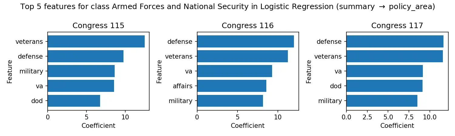
The model learns interpretable features for each policy area. For example, Agriculture bills are strongly associated with terms like “farm,” “crop,” and “livestock,” while Armed Forces bills correlate with “military,” “defense,” and “veterans.”

Naive Bayes Top Features for Agriculture and Food

Naive Bayes Top Features for Armed Forces and National Security

Naive Bayes Top Features for Arts, Culture, Religion

Naive Bayes Top Features for Civil Rights and Liberties, Minority Issues

Naive Bayes Top Features for Crime and Law Enforcement

Naive Bayes Top Features for Economics and Public Finance

Naive Bayes Top Features for Emergency Management

Naive Bayes Top Features for Environmental Protection

Naive Bayes Top Features for Finance and Financial Sector

Naive Bayes Top Features for Foreign Trade and International Finance

Naive Bayes Top Features for Government Operations and Politics

Naive Bayes Top Features for Housing and Community Development

Naive Bayes Top Features for International Affairs

Naive Bayes Top Features for Labor and Employment

Naive Bayes Top Features for Native Americans

Naive Bayes Top Features for Public Lands and Natural Resources

Naive Bayes Top Features for Science, Technology, Communications

Naive Bayes Top Features for Social Sciences and History

Naive Bayes Top Features for Social Welfare

Naive Bayes Top Features for Sports and Recreation

Naive Bayes Top Features for Transportation and Public Works

Naive Bayes Top Features for Water Resources Development

Naive Bayes Top Features for Private Legislation

Logistic Regression

Title-only Logistic Regression experiments are run with the following settings:

sweep_logreg(
    data,
    X_key='title',
    y_key='policy_area',
    tfidf_params={
        'lowercase': True,
        'dtype': np.float32,
    },
    tfidf_grid={
        'ngram_range': [(1, 1), (1, 2)],
        'max_df': (0.05, 0.1, 0.25),
    },
    logreg_params={
        'max_iter': 1000,
        'random_state': 42,
        'class_weight': 'balanced',
    },
    logreg_grid={
        'C': [0.1, 1, 10],
    },
)

and the results:

Training on Congress 115
Best score: 0.704
Refit Time: 32.063
Best parameters set:
	clf__C: 10
	tfidf__max_df: 0.05
	tfidf__ngram_range: (1, 2)
Testing on Congress 116 F1: 0.6809188275881766
Testing on Congress 117 F1: 0.601917336933838

Training on Congress 116
Best score: 0.714
Refit Time: 31.227
Best parameters set:
	clf__C: 10
	tfidf__max_df: 0.05
	tfidf__ngram_range: (1, 2)
Testing on Congress 115 F1: 0.7408989977276476
Testing on Congress 117 F1: 0.7200639105208106

Training on Congress 117
Best score: 0.711
Refit Time: 34.083
Best parameters set:
	clf__C: 10
	tfidf__max_df: 0.05
	tfidf__ngram_range: (1, 2)
Testing on Congress 115 F1: 0.674418393892329
Testing on Congress 116 F1: 0.7405934743144291

Mean fit time: 32.46 ± 1.20s

Results Summary

Logistic regression improves upon Naive Bayes performance:

Higher F1 scores: Generally 5-7 percentage points better than Naive Bayes
Consistent hyperparameters: Optimal settings remain stable across Congresses
Reasonable training time: 30-35 seconds per model remains manageable
Strong cross-Congress generalization: F1 scores consistently above 0.70

Logistic Regression Policy Area Classification F1 Score

XGBoost

Title-only XGBoost experiments are run with the following settings:

sweep_xgb(
    data,
    X_key='title',
    y_key='policy_area',
    tfidf_grid={
        'max_df': (0.05,),
    },
    xgb_grid={
        'max_depth': (6,),
        'eta': (0.3,),
    },
)

and the results:

Training on Congress 115
Best score: 0.591
Refit Time: 198.063
Best parameters set:
	clf__eta: 0.3
	clf__max_depth: 6
	clf__num_class: 33
	tfidf__max_df: 0.05
Testing on Congress 116 F1: 0.5649530686141018
Testing on Congress 117 F1: 0.5215939580735101

Training on Congress 116
Best score: 0.600
Refit Time: 264.824
Best parameters set:
	clf__eta: 0.3
	clf__max_depth: 6
	clf__num_class: 33
	tfidf__max_df: 0.05
Testing on Congress 115 F1: 0.6037922738570368
Testing on Congress 117 F1: 0.5965027418245722

Training on Congress 117
Best score: 0.595
Refit Time: 249.799
Best parameters set:
	clf__eta: 0.3
	clf__max_depth: 6
	clf__num_class: 33
	tfidf__max_df: 0.05
Testing on Congress 115 F1: 0.5600491477899472
Testing on Congress 116 F1: 0.60815381664894

Mean fit time: 237.56 ± 28.60s

Results Summary

XGBoost underperforms relative to expectations:

Poor performance: F1 scores significantly below linear models (0.55-0.60 range)
Long training times: 4+ minutes per model with limited hyperparameter exploration
Questionable value: The computational cost doesn’t justify the poor performance

Given these results, we focus on the more promising linear models for subsequent experiments with longer text inputs.

XGBoost Policy Area Classification F1 Score

Training Efficiency

The computational costs vary dramatically:

Model	Training Time
Naive Bayes	0.54 ± 0.03s
Logistic Regression	32.46 ± 1.20s
XGBoost	237.56 ± 28.60s

XGBoost’s poor performance despite high computational cost suggests that tree-based methods may not be well-suited for sparse TF-IDF features. We’ll focus on linear models for the remaining experiments.

Summary-Only Results

Using bill summaries provides substantially more context than titles alone, leading to significant performance improvements.

Naive Bayes Performance

The summary-based models show dramatic improvement over title-only versions:

F1 scores: 0.85+ within-Congress, 0.77-0.86 cross-Congress
Training time: Still fast at ~3.4 seconds
Strong generalization: Consistent performance across time periods

Naive Bayes Summary Performance — Summary-based models achieve 80%+ F1 scores across most Congress combinations

Logistic Regression Performance

Logistic regression slightly outperforms Naive Bayes on summaries:

F1 scores: 0.86+ within-Congress, 0.79-0.87 cross-Congress
Training time: Reasonable at ~12 seconds
Stable hyperparameters: Consistent optimal settings across Congresses

The performance difference between models suggests they rely on similar feature patterns, with logistic regression better capturing feature interactions.

Logistic Regression

Summary-only Logistic Regression experiments are run with the following settings:

sweep_logreg(
    data,
    X_key='summary',
    y_key='policy_area',
    tfidf_params={
        'lowercase': True,
        'dtype': np.float32,
    },
    tfidf_grid={
        # 'ngram_range': [(1, 1), (1, 2)],
        'max_df': (0.05, 0.1, 0.25),
    },
    logreg_params={
        'max_iter': 1000,
        'random_state': 42,
        'class_weight': 'balanced',
    },
    logreg_grid={
        'C': [0.1, 1, 10],
    },
)

And the results:

Training on Congress 115
Best score: 0.862
Refit Time: 9.007
Best parameters set:
	clf__C: 10
	tfidf__max_df: 0.25
Testing on Congress 116 F1: 0.8284864693401133
Testing on Congress 117 F1: 0.7934161507811646

Training on Congress 116
Best score: 0.865
Refit Time: 13.897
Best parameters set:
	clf__C: 10
	tfidf__max_df: 0.25
Testing on Congress 115 F1: 0.8637852557418315
Testing on Congress 117 F1: 0.8594775615031977

Training on Congress 117
Best score: 0.862
Refit Time: 12.167
Best parameters set:
	clf__C: 10
	tfidf__max_df: 0.25
Testing on Congress 115 F1: 0.8355736563084967
Testing on Congress 116 F1: 0.8696403838390832

Mean fit time: 11.69 ± 2.02s

Full Text Results

We test whether complete bill text improves performance over summaries, using optimal hyperparameters from summary experiments.

Naive Bayes on Full Text

Surprisingly, full text yields slightly lower performance than summaries:

F1 scores: 0.84-0.85 within-Congress, 0.77-0.86 cross-Congress
Training time: ~50 seconds (10× slower than summaries)
Performance drop: Likely due to increased noise in lengthy documents

Naive Bayes Full Text Performance — Full text performance is slightly worse than summaries, suggesting diminishing returns

Logistic Regression on Full Text

Logistic regression shows the strongest performance on full text:

F1 scores: 0.87-0.88 within-Congress, 0.83-0.89 cross-Congress
Training time: ~70 seconds
Best overall performance: Approaches 90% F1 on some Congress pairs

Logistic Regression Full Text Performance — Logistic regression achieves the best performance using full bill text

The logistic regression model benefits from having access to complete legislative language while effectively regularizing against noise.

Key Findings

This baseline study establishes several important results:

Best performing model: Logistic regression trained on full bill text achieves up to 89% F1 score, providing a strong benchmark for future deep learning approaches.

Text input comparison:

Titles: Limited but fast (F1 ~0.65-0.70)
Summaries: Good balance of performance and efficiency (F1 ~0.85)
Full text: Best performance but computationally expensive (F1 ~0.87-0.89)

Cross-Congress generalization: Models trained on one Congress generalize reasonably well to others, though performance decreases with temporal distance between sessions.

Model performance ranking: Logistic Regression > Naive Bayes » XGBoost for this text classification task.

Next Steps

The strong baseline performance sets the stage for several research directions:

Deep learning models: Transformer-based approaches using pre-trained language models
Dataset expansion: Including additional Congresses and more detailed bill metadata
Error analysis: Understanding failure cases and class-specific performance patterns
Feature engineering: Exploring domain-specific text preprocessing and feature extraction

The complete dataset and experimental code are available for researchers interested in building upon these baselines.

Resources:

Dataset: Hugging Face: hheiden/us-congress-bill-policy-115_117
Leaderboard: Policy Area Classification Leaderboard

Introduction#

Why This Matters#

Data#

Bills by Congress#

Policy Areas#

Text Statistics#

Evaluation Framework#

Experimental Design#

Metrics and Hyperparameter Tuning#

Baseline Models#

Text Preprocessing#

Multinomial Naive Bayes#

Logistic Regression#

XGBoost#

Results#

Title-Only Inputs#

Naive Bayes#

Results Summary#

Logistic Regression#

Results Summary#

XGBoost#

Results Summary#

Training Efficiency#

Summary-Only Results#

Naive Bayes Performance#

Logistic Regression Performance#

Logistic Regression#

Full Text Results#

Naive Bayes on Full Text#

Logistic Regression on Full Text#

Key Findings#

Next Steps#

Introduction

Why This Matters

Data

Bills by Congress

Policy Areas

Text Statistics

Evaluation Framework

Experimental Design

Metrics and Hyperparameter Tuning

Baseline Models

Text Preprocessing

Multinomial Naive Bayes

Logistic Regression

XGBoost

Results

Title-Only Inputs

Naive Bayes

Results Summary

Logistic Regression

Results Summary

XGBoost

Results Summary

Training Efficiency

Summary-Only Results

Naive Bayes Performance

Logistic Regression Performance

Logistic Regression

Full Text Results

Naive Bayes on Full Text

Logistic Regression on Full Text

Key Findings

Next Steps