Introduction
Can you determine a molecule’s shape from mathematical fingerprints alone? This question drives some of the most fundamental challenges in computational chemistry and machine learning. In the broader ML context, this is the classic search for the right inductive bias or invariant representation. Whether we are processing messy documents, natural language, or molecular dynamics, finding a representation that captures essential structure while ignoring irrelevant variations is critical.
I recently encountered a paper with an intriguing title: “Can One Hear the Shape of a Molecule (from its Coulomb Matrix Eigenvalues)?” The title references Mark Kac’s famous mathematical question “Can One Hear the Shape of a Drum?” exploring whether a drum’s shape dictates its sound frequencies.
The molecular version asks: can we determine a molecule’s structure from the eigenvalues of its Coulomb matrix?
Molecular representations are the foundation of machine learning in chemistry. If eigenvalues can capture structural information, they become powerful features for property prediction. Successfully separating simple structural differences is a prerequisite for handling more complex molecules.
The original authors tested this hypothesis using alkane constitutional isomers (molecules with identical formulas but different structural arrangements). I decided to replicate and extend their work to better understand both the methods and their limitations.
In this post, we will explore molecular representation through eigenvalue analysis, covering data generation, unsupervised clustering approaches, and supervised classification methods. I’ll also explore log-transformed Coulomb matrices, which can reveal structural details that standard matrices miss.
Why Alkanes Make Ideal Test Cases
Alkanes are the simplest organic molecules: carbon and hydrogen connected by single bonds with the general formula $C_{n}H_{2n+2}$.
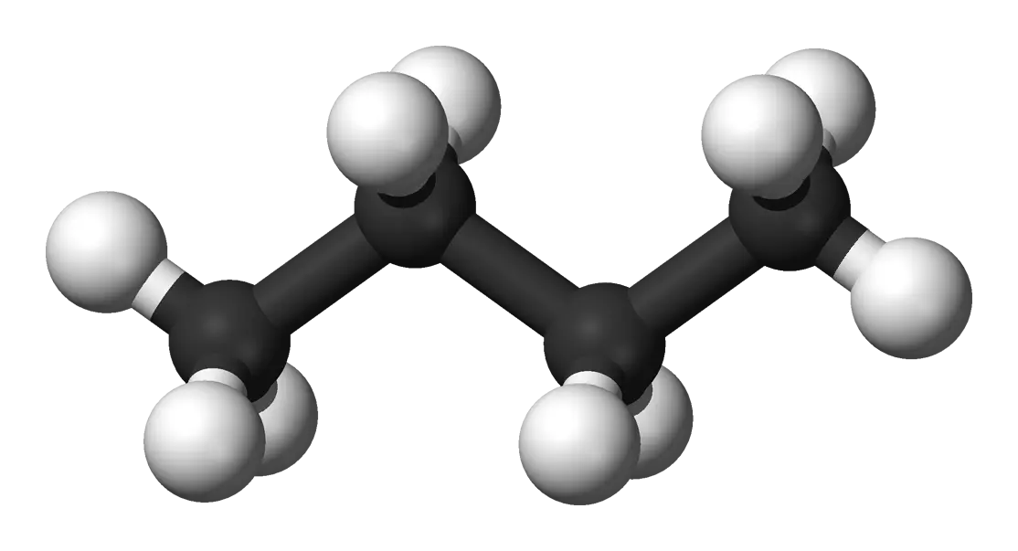
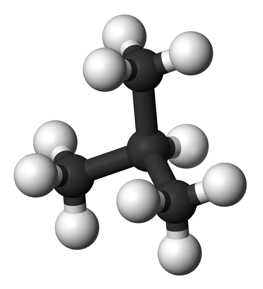
What makes them perfect for testing molecular representations is their constitutional isomers: molecules with identical formulas but different structural arrangements. For small alkanes ($n \leq 3$), atoms can connect in only one way. Starting with butane ($n = 4$), multiple arrangements become possible:

The number of isomers grows rapidly with molecular size. By undecane ($n = 11$), there are 159 different structural arrangements:
| Alkane | n | Isomers |
|---|---|---|
| Butane | 4 | 2 |
| Pentane | 5 | 3 |
| Hexane | 6 | 5 |
| Heptane | 7 | 9 |
| Octane | 8 | 18 |
| Nonane | 9 | 35 |
| Decane | 10 | 75 |
| Undecane | 11 | 159 |
This creates a natural classification challenge: can Coulomb matrix eigenvalues distinguish these structural differences? Successfully separating simple alkane isomers is a prerequisite for handling more complex molecules.
Computational Pipeline
The analysis requires three computational steps:
- Generate constitutional isomers for each alkane formula
- Create multiple 3D conformations for each isomer
- Calculate Coulomb matrix eigenvalues for each conformation
Generating Constitutional Isomers
Enumerating all possible carbon skeletons is a combinatorial problem. I used MAYGEN, an open-source Java tool for generating molecular structures from chemical formulas.
For butane ($C_{4}H_{10}$):
java -jar MAYGEN-1.8.jar -v -m -f C4H10 -smi -o butane_conformers.smi
This generates:
CCCC
CC(C)C
The first is n-butane (linear), the second is isobutane (branched). We can automate this across all alkanes:
os.makedirs('isomers', exist_ok=True)
for n in range(1, 12):
    cmd = f"java -jar MAYGEN-1.8.jar -f C{n}H{2*n + 2} -smi -o isomers/C{n}H{2*n + 2}.smi"
    os.system(cmd)
Generating 3D Conformations
For machine learning applications, we need multiple 3D structures of each isomer to capture conformational flexibility. I used RDKit’s ETKDG method, which remains competitive with commercial alternatives:
from rdkit.Chem import AllChem


def smiles_str_to_rdkit_mol(smiles_str: str) -> rdkit.Chem.Mol:
    """Convert a SMILES string to an RDKit mol object.

    Args:
    - smiles_str (str): A SMILES string representing a molecule.

    Returns:
    - mol (rdkit.Chem.Mol): An RDKit mol object representing the molecule.
    """

    # Convert SMILES string to RDKit mol object
    mol = rdkit.Chem.MolFromSmiles(smiles_str)

    # Add hydrogens to the molecule
    mol = rdkit.Chem.AddHs(mol)

    # Assign 3D coordinates to the molecule
    AllChem.EmbedMolecule(mol)

    return mol
Computing Coulomb Matrix Eigenvalues
The Coulomb matrix encodes 3D structure in a rotation and translation-invariant way. Its eigenvalues should capture structural information while remaining invariant to molecular orientation.
First, I wrote a helper function to convert RDKit molecules into ASE Atoms objects that DScribe can process:
def rdkit_mol_to_ase_atoms(rdkit_mol: rdkit.Chem.Mol) -> ase.Atoms:
    """Convert an RDKit molecule to an ASE Atoms object.

    Args:
        rdkit_mol: RDKit molecule object.

    Returns:
        ASE Atoms object.
    """
    ase_atoms = ase.Atoms(
        numbers=[
            atom.GetAtomicNum() for atom in rdkit_mol.GetAtoms()
        ],
        positions=rdkit_mol.GetConformer().GetPositions()
    )
    return ase_atoms
Then I computed Coulomb matrix eigenvalues using DScribe, with optional log transformation:
def ase_atoms_to_coloumb_matrix_eigenvalues(
    ase_atoms: ase.Atoms,
    log: bool = False
) -> np.ndarray:
    """Convert an ASE Atoms object to a Coulomb matrix and calculate its eigenvalues.

    Args:
        ase_atoms: ASE Atoms object.
        log: Whether to log transform the Coulomb matrix prior to calculating the eigenvalues.

    Returns:
        Eigenvalues of the Coulomb matrix.
    """
    # Create a Coulomb matrix
    coulomb_matrix = dscribe.descriptors.CoulombMatrix(
        n_atoms_max=ase_atoms.get_global_number_of_atoms(),
    )

    # Calculate the Coulomb matrix
    coulomb_matrix = coulomb_matrix.create(ase_atoms)
    coulomb_matrix = coulomb_matrix.reshape(
        ase_atoms.get_global_number_of_atoms(),
        ase_atoms.get_global_number_of_atoms())

    if log:
        # Log transform the Coulomb matrix
        coulomb_matrix = np.log(coulomb_matrix)

    # Calculate the eigenvalues of the Coulomb matrix
    eigenvalues = np.linalg.eigvals(coulomb_matrix)
    return eigenvalues
Combining these functions enables efficient data generation:
# Generate 1000 conformations per isomer for each alkane
# gen_n_spectra() combines the above functions to generate multiple conformations
os.makedirs('spectra', exist_ok=True)
n_confs = 1000

for n in range(1, 12):
    print(f'Generating spectra for C{n}H{2*n + 2}')

    with open(f'isomers/C{n}H{2*n + 2}.smi') as f:
        smiles_list = [line.strip() for line in f]

    for i, smiles in enumerate(smiles_list):
        spectra = gen_n_spectra(smiles, n_confs, log=False)
        np.save(f'spectra/C{n}H{2*n + 2}_{i}.npy', spectra)
Reproducing the Original Results
To validate our computational pipeline, I replicated key figures from the original paper. This ensures our implementation correctly captures the phenomena they observed.
We generate data using 1000 conformations per isomer:
os.makedirs('spectra', exist_ok=True)

n_confs = 1000
for n in range(1, 12):
    print(f'Generating spectra for C{n}H{2*n + 2}')
    with open(f'isomers/C{n}H{2*n + 2}.smi') as f:
        lines = f.readlines()
        for i, line in enumerate(lines):
            if not line.strip():
                continue

            smiles = line.strip()
            spectra = gen_n_spectra(n_confs, smiles, log=False)
            np.save(f'spectra/C{n}H{2*n + 2}_{i:03d}.npy', spectra)
After generation, we can load the data into a structured format:
import re
from glob import glob

spectra = {}
for n in range(1, 12):
    spectra[n] = {}
    for f in glob(f'spectra/C{n}H{2*n + 2}_*.npy'):
        j = int(re.search(rf'C{n}H{2*n + 2}_(\d+).npy', f).group(1))
        spectra[n][j] = np.load(f)
Largest Eigenvalues Across Alkane Series
The first analysis examines how the largest Coulomb matrix eigenvalues vary across constitutional isomers for each alkane formula. This plot reveals whether single eigenvalues can distinguish between different molecular formulas.
fig, ax = plt.subplots(1, 1, figsize=(10, 5))

for n in range(1, 12):
    eigenvalues = np.array([spectra[n][i][:, 0].mean() for i in spectra[n]])

    # add black dots to boxplot, but not dirextly to the center line
    jitter = np.random.normal(0, 0.1, size=len(eigenvalues))
    ax.scatter(np.full(len(eigenvalues), n) + jitter, eigenvalues, color='black', s=1, alpha=0.3)

    # Plot median
    ax.scatter([n], [np.median(eigenvalues)], color='red', alpha=0.5)

    # Plot range
    ax.plot([n - 0.5, n + 0.5], [np.min(eigenvalues), np.min(eigenvalues)], 'k-', alpha=0.5)
    ax.plot([n - 0.5, n + 0.5], [np.max(eigenvalues), np.max(eigenvalues)], 'k-', alpha=0.5)

ax.set_xlabel('Molecular formula')
ax.set_ylabel('Largest eigenvalue')
ax.set_xticks(range(1, 12))
ax.set_xticklabels([f'C{n}H{2*n + 2}' for n in range(1, 12)])
ax.set_title('Largest eigenvalues of the Coulomb matrix for alkane constitutional isomers')
plt.savefig('alkane_coulomb_matrix_largest_eigenvalues.webp', bbox_inches='tight')
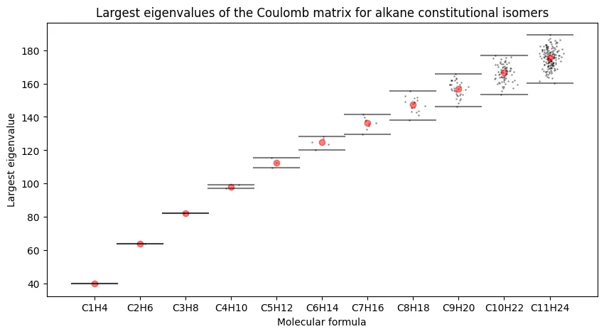
Our results match the original paper. We observe sub-linear growth in the largest eigenvalue with carbon number, and critically, increasing overlap between isomers as molecules grow larger. The largest eigenvalue alone cannot reliably distinguish constitutional isomers for larger alkanes.
Eigenvalue Distributions for Heptane Isomers
Looking deeper at a specific case, I analyzed the probability density functions for heptane ($C_7H_{16}$) isomers. This molecule has nine constitutional isomers, providing a good test of discrimination power.
for n_sel in range(4, 8):
    fig, ax = plt.subplots(1, 1, figsize=(10, 5))

    smiles = []
    with open(f'isomers/C{n_sel}H{2*n_sel + 2}.smi') as f:
        for line in f:
            smiles.append(line.strip())

    for i in range(len(spectra[n_sel])):
        eigenvalues = spectra[n_sel][i][:, 0]

        # kde plot with the following params
        # - Gaussian kernel
        # - bandwidth with Silverman's rule of thumb
        ax = sns.kdeplot(eigenvalues, bw_method='silverman', label=get_iupac_name(smiles[i]))

    ax.set_xlabel('Largest eigenvalue')
    ax.set_ylabel('Density')
    ax.set_title('PDF of the largest eigenvalue for $C_' + str(n_sel) + 'H_{' + str(2*n_sel + 2) + '}$')
    ax.legend()
    plt.savefig(f'pdf_largest_eigenvalue_C{n_sel}H{2*n_sel + 2}.webp', bbox_inches='tight')
    plt.close()
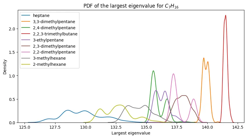
The pattern is clear:
- n-heptane (linear chain) has the smallest eigenvalues
- 2,2,3-trimethylbutane (highly branched) has the largest
- Seven other isomers fall in between with substantial overlap
This demonstrates the fundamental limitation: while extreme structural differences (linear vs. highly branched) create separable eigenvalue distributions, intermediate structures become indistinguishable.
For smaller alkanes, the separation is more promising:
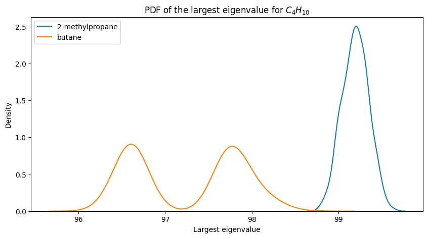
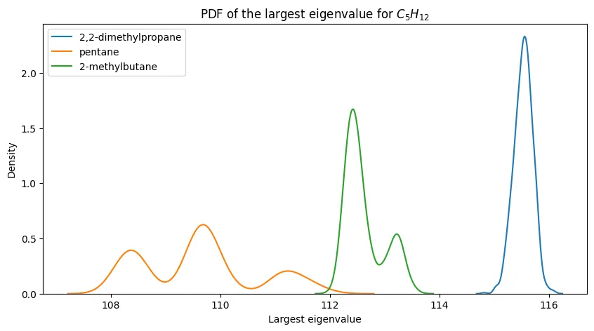
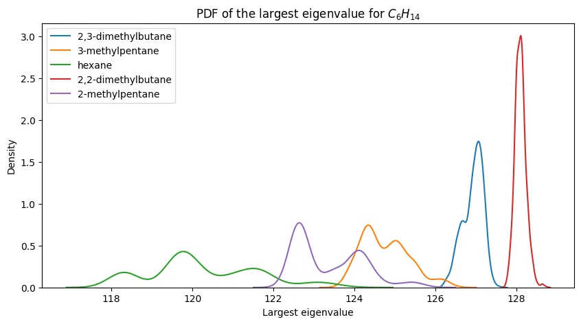
The progression is clear: eigenvalue-based discrimination works well for small alkanes and degrades as molecular complexity increases.
Two-Dimensional Eigenvalue Space
Can we improve discrimination by using multiple eigenvalues? For butane, plotting the first two eigenvalues reveals interesting structure:
fig, ax = plt.subplots(1, 1, figsize=(10, 5))

n_sel = 4
smiles = []
with open(f'isomers/C{n_sel}H{2*n_sel + 2}.smi') as f:
    for line in f:
        smiles.append(line.strip())

for i in range(len(spectra[n_sel])):
    eigenvalues = spectra[n_sel][i][:, :2]

    ax.scatter(eigenvalues[:, 0], eigenvalues[:, 1], label=get_iupac_name(smiles[i]))

ax.set_xlabel('Largest eigenvalue')
ax.set_ylabel('Second largest eigenvalue')
ax.set_title('2D plot of the first two eigenvalues for $C_4H_{10}$ conformers')
ax.legend()
plt.savefig(f'2d_largest_eigenvalue_C{n_sel}H{2*n_sel + 2}.webp', bbox_inches='tight')
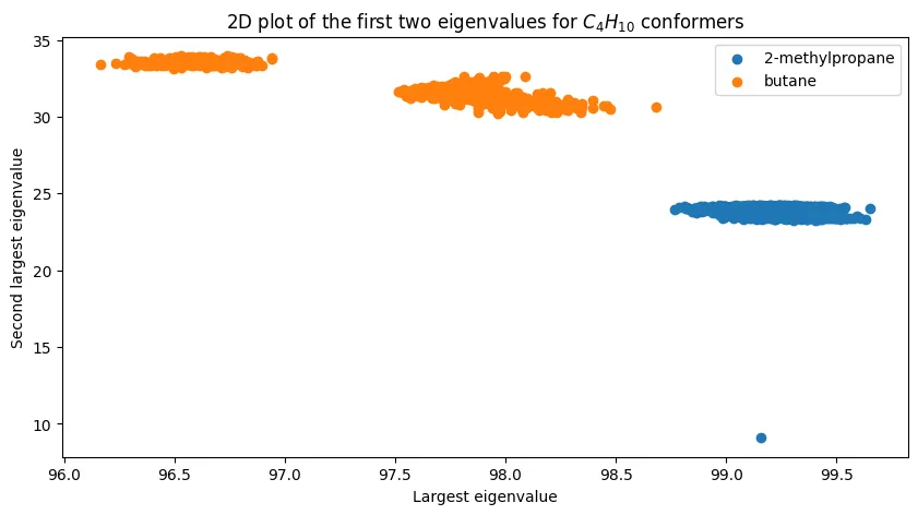
The two isomers cluster distinctly, demonstrating that multi-dimensional eigenvalue features can achieve perfect separation for simple cases. The outlier point in the lower right likely results from conformational sampling noise.
Dimensionality and Information Content
How many eigenvalues do we actually need? Principal component analysis reveals the effective dimensionality of the eigenvalue representations:
from sklearn.decomposition import PCA

fig, ax = plt.subplots(1, 1, figsize=(10, 5))

n_components = {}
for n in range(1, 12):
    n_components[n] = []

    for i in range(len(spectra[n])):
        eigenvalues = spectra[n][i]

        # PCA
        pca = PCA(n_components=0.99, svd_solver='full', whiten=False, random_state=42)
        pca.fit(eigenvalues)
        n_components[n].append(pca.n_components_)

    ax.scatter([n] * len(n_components[n]), n_components[n], alpha=0.3)
    ax.plot([n - 0.25, n + 0.25], [np.mean(n_components[n]), np.mean(n_components[n])], 'k-', alpha=0.5)  # Draw a line for the mean

ax.plot([1, 11], [1, 11], 'k--', alpha=0.5, label='y = num carbon')
ax.plot([1, 11], [5, 35], 'r--', alpha=0.5, label='y = num atoms')

ax.set_xlabel('Number of carbon atoms')
ax.set_ylabel('Number of principal components')
ax.set_title('99% variance explained by number of principal components')
plt.legend()
plt.savefig('99_variance_explained.webp', bbox_inches='tight')
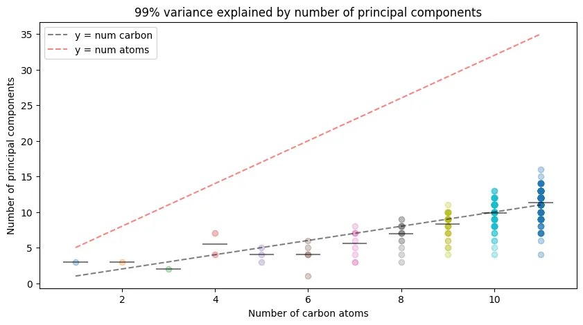
Key observations:
- High compressibility: Much fewer than the $3n+2$ degrees of freedom are needed
- Linear scaling: Principal components grow roughly linearly with carbon number
- Efficient representation: The eigenvalue space has lower effective dimensionality than expected
This suggests the representations are highly correlated, enabling significant dimensionality reduction without information loss.
Log-Transformed Coulomb Matrices
As explored in our previous post on Coulomb matrices, log transformation can reveal different structural information. Standard Coulomb matrices emphasize heavy atom interactions. Log transformation expands the influence of hydrogen atoms by mapping magnitudes in $[0,1]$ to $[-\infty,0]$.
I generated equivalent datasets using log-transformed matrices to test how this affects discriminative power.
os.makedirs('spectra', exist_ok=True)

n_confs = 1000
for n in range(1, 12):
    print(f'Generating spectra for C{n}H{2*n + 2}')
    with open(f'isomers/C{n}H{2*n + 2}.smi') as f:
        lines = f.readlines()
        print(f'\tNumber of SMILES strings: {len(lines)}')
        for i, line in enumerate(tqdm(lines)):
            print(f'\t\t{i + 1}/{len(lines)} - {line.strip()}')

            if not line.strip():
                continue

            if os.path.exists(f'spectra/log-C{n}H{2*n + 2}_{i}.npy'):
                continue

            smiles = line.strip()
            spectra = gen_n_spectra(n=n_confs, smiles_str=smiles, log=True)
            np.save(f'spectra/log-C{n}H{2*n + 2}_{i:03d}.npy', spectra)
Log-Transformed Eigenvalue Distributions
The log transformation dramatically changes the eigenvalue landscape:
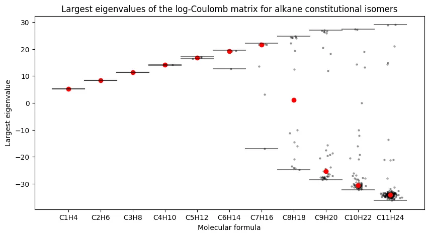
Log-transformed versions exhibit distinct characteristics:
- Span large negative values due to hydrogen atom emphasis
- Show increasing variance between isomers as molecular size grows
- Demonstrate greater discrimination potential for some isomers
This comes with trade-offs. The distributions can become significantly broader, as seen in the heptane analysis:
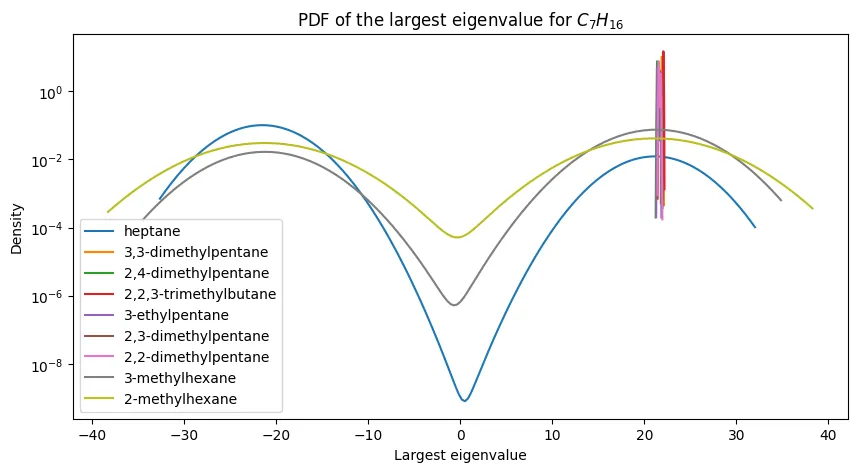
The log scale on the y-axis is necessary because unbranched isomers become nearly invisible due to the highly concentrated distributions of branched isomers.
Two-Dimensional Log-Transformed Space
The 2D eigenvalue plot for log-transformed butane shows similar clustering behavior:
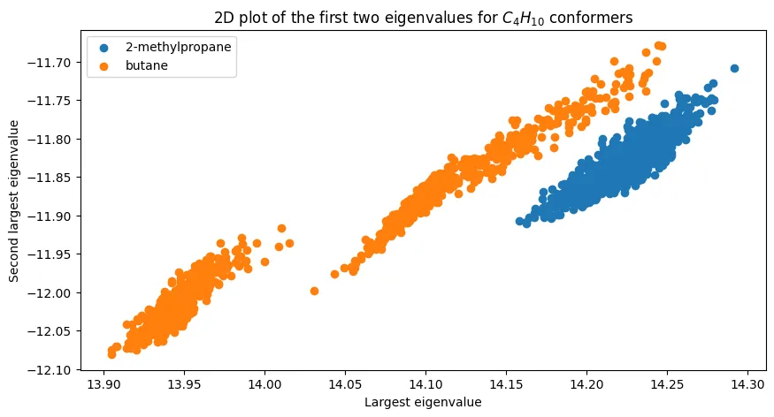
The transformation reduces the separation distance, yet linear discriminability remains intact for this simple case.
Dimensionality of Log-Transformed Features
Principal component analysis of log-transformed eigenvalues reveals similar compression properties:
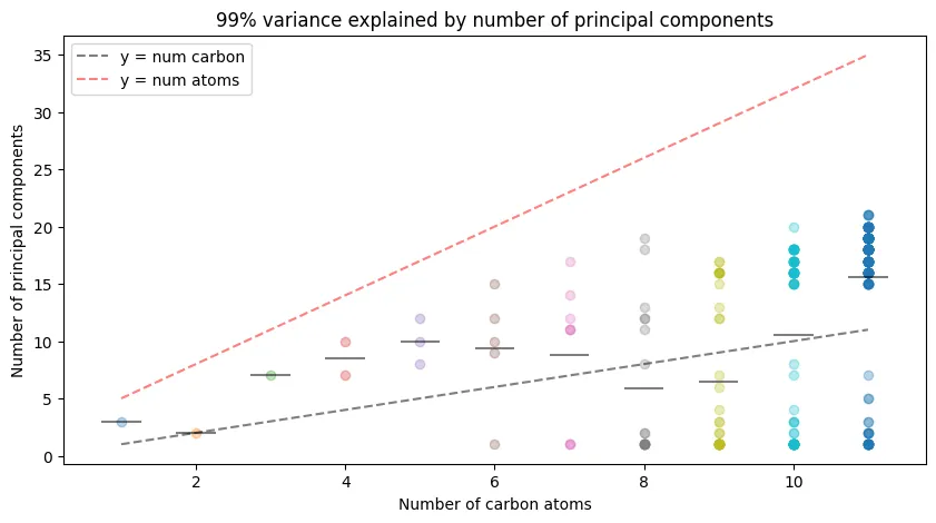
The log-transformed features show comparable dimensionality reduction with marginally higher component requirements.
Testing Eigenvalue Separability
Our exploratory analysis revealed concerning patterns that hint at fundamental limitations: high correlation between eigenvalue dimensions, rapid dimensionality compression via PCA, and overlapping distributions for larger molecules ($n \geq 6$).
These findings leave the question open. We now test eigenvalues directly to see if they can actually separate constitutional isomers without supervision.
We’ll use two complementary clustering metrics to measure how well eigenvalues separate constitutional isomers. This is a fair test. We only compare isomers with identical molecular formulas, keeping eigenvalue dimensions constant.
Dunn Index: Global Cluster Quality
The Dunn Index provides a single metric capturing cluster quality. It asks: “Are the closest different clusters still farther apart than the most spread-out individual cluster?”
$$ \text{Dunn Index} = \frac{\text{smallest distance between different clusters}}{\text{largest diameter within any cluster}} $$
Higher values indicate better separation. When it approaches zero, clusters become indistinguishable, exactly what we suspected from the overlapping eigenvalue distributions observed earlier.
Computing the Dunn Index for each alkane series:
import time

dunn_scores = {}
for n in range(4, 12):
    tik = time.time()
    dunn_scores[n] = dunn_index([spectra[n][i] for i in spectra[n]])
    tok = time.time()
    dunn_scores[n]['time'] = tok - tik
    print(f'C{n}H{2*n + 2}:', dunn_scores[n])
C4H10: {'diameter': 21.43072917950398, 'distance': 8.316362440688767, 'dunn_index': 0.3880578383978837, 'time': 0.06010293960571289}
C5H12: {'diameter': 23.449286379564892, 'distance': 2.4693042873545856, 'dunn_index': 0.10530402705587172, 'time': 0.10832405090332031}
C6H14: {'diameter': 19.602363375467938, 'distance': 1.4477574259511048, 'dunn_index': 0.07385626917634591, 'time': 0.28030991554260254}
C7H16: {'diameter': 20.065014927470955, 'distance': 0.4050094394280803, 'dunn_index': 0.02018485612355977, 'time': 1.0307331085205078}
C8H18: {'diameter': 24.794154667613665, 'distance': 0.5013450168168625, 'dunn_index': 0.020220290771668196, 'time': 4.199508905410767}
C9H20: {'diameter': 21.811025941686033, 'distance': 0.34381162248560415, 'dunn_index': 0.01576320267578513, 'time': 17.400264978408813}
C10H22: {'diameter': 27.180773716656066, 'distance': 0.4986608768730121, 'dunn_index': 0.0183460883811206, 'time': 86.00787401199341}
C11H24: {'diameter': 25.58731511020692, 'distance': 0.5490373275460223, 'dunn_index': 0.021457402825629343, 'time': 424.4431610107422}
The computation time grows dramatically, over 7 minutes for $C_{11}H_{24}$, due to quadratic scaling with the number of isomers (159 isomers requiring ~12,000 pairwise comparisons).
The results reveal a clear trend:
fig, axs = plt.subplots(2, 2, figsize=(15, 10))

# in axs[0, 0] - diameter vs number of carbon atoms
axs[0, 0].plot(
    list(range(4, 12)),
    [dunn_scores[n]['diameter'] for n in range(4, 12)],
    marker='o'
)
axs[0, 0].set_xlabel('Number of carbon atoms')
axs[0, 0].set_ylabel('Diameter')
axs[0, 0].set_title('Diameter vs number of carbon atoms')

# in axs[0, 1] - distance vs number of carbon atoms
axs[0, 1].plot(
    list(range(4, 12)),
    [dunn_scores[n]['distance'] for n in range(4, 12)],
    marker='o'
)
axs[0, 1].set_xlabel('Number of carbon atoms')
axs[0, 1].set_ylabel('Distance')
axs[0, 1].set_title('Distance vs number of carbon atoms')

# in axs[1, 0] - dunn index vs number of carbon atoms
axs[1, 0].plot(
    list(range(4, 12)),
    [dunn_scores[n]['dunn_index'] for n in range(4, 12)],
    marker='o'
)
axs[1, 0].set_xlabel('Number of carbon atoms')
axs[1, 0].set_ylabel('Dunn index')
axs[1, 0].set_title('Dunn index vs number of carbon atoms')

# in axs[1, 1] - time vs number of carbon atoms
axs[1, 1].plot(
    list(range(4, 12)),
    [dunn_scores[n]['time'] for n in range(4, 12)],
    marker='o'
)
axs[1, 1].set_xlabel('Number of carbon atoms')
axs[1, 1].set_ylabel('Time (s)')
axs[1, 1].set_title('Time vs number of carbon atoms')

plt.tight_layout()
plt.savefig('dunn_index_vs_num_carbon_atoms.webp', bbox_inches='tight')
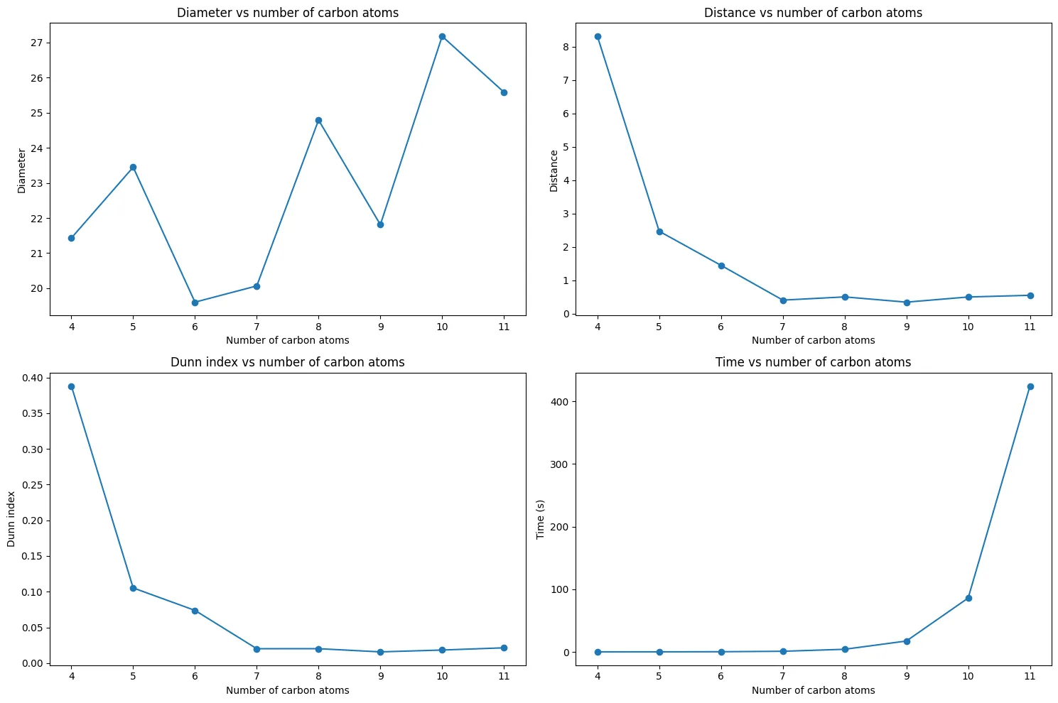
The trend confirms our earlier concerns:
- $C_{4}H_{10}$: Excellent separation (Dunn Index = 0.39) between butane and isobutane
- $C_{5}H_{12}$ to $C_{6}H_{14}$: Rapid decline in separability
- $C_{7}H_{16}$ and beyond: Poor separation (Dunn Index $\approx$ 0.02)
This validates our computational pipeline and matches the original paper’s findings. For larger molecules, eigenvalue clusters become nearly indistinguishable, confirming the overlapping distributions we observed earlier.
Silhouette Analysis: Individual Conformation Assessment
The Dunn Index provides the global view. We must also consider individual molecules. The silhouette score evaluates each conformation separately, asking: “Is this molecule closer to its own isomer family or to a different one?”
For each molecular conformation $i$:
$$ s(i) = \frac{b(i) - a(i)}{\max(a(i), b(i))} $$
where:
- $a(i)$ = average distance to other conformations of the same isomer
- $b(i)$ = average distance to conformations of the nearest different isomer
Interpretation:
- Score near +1: Conformation clusters correctly (good clustering)
- Score near -1: Conformation closer to different isomer (misclassification)
This enables two critical measurements:
- How many isomers have any misclassified conformations?
- What fraction of individual conformations get misclassified?
from sklearn.metrics import silhouette_samples
from tqdm import tqdm

s_scores = {}
for n in tqdm(range(4, 12)):
    X = []
    y = []
    for i in spectra[n]:
        X.append(spectra[n][i])
        y.extend(np.full(spectra[n][i].shape[0], i))
    X = np.concatenate(X)
    y = np.array(y)

    s_scores[n] = silhouette_samples(X, y)
Computing both clustering quality metrics:
# Metric 1: Fraction of isomers with ANY negative scores
neg_iso = {}
for n in range(4, 12):
    n_iso = s_scores[n].shape[0] // 1000
    n_has_neg = 0
    for i in range(n_iso):
        chunk = s_scores[n][i * 1000:(i + 1) * 1000]
        if np.any(chunk < 0):
            n_has_neg += 1
    neg_iso[n] = n_has_neg / n_iso

# Metric 2: Individual conformation misclassification rates
neg_confs = {}
for n in range(4, 12):
    n_iso = s_scores[n].shape[0] // 1000
    neg_confs[n] = np.zeros(n_iso)
    for i in range(n_iso):
        isomer_scores = s_scores[n][i * 1000:(i + 1) * 1000]
        neg_confs[n][i] = np.sum(isomer_scores < 0) / isomer_scores.shape[0]
Isomer-Level Analysis
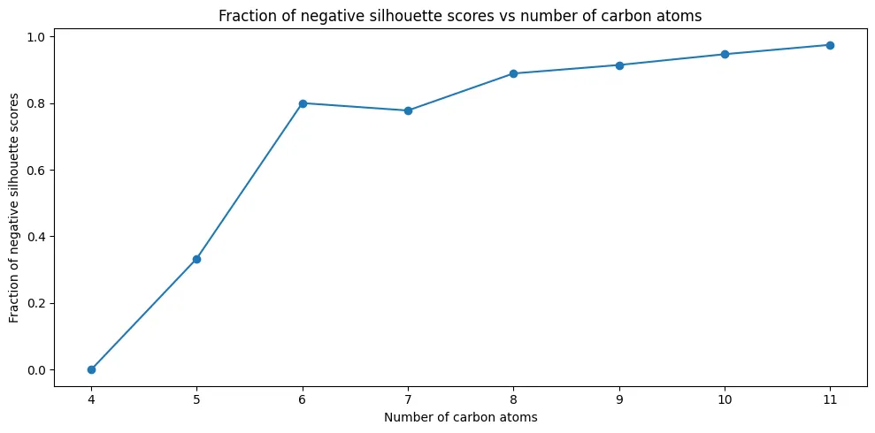
The trend is concerning: by $C_{11}H_{24}$, 97% of isomers have at least one conformation that would be misclassified. This metric is deliberately strict. Even a single misplaced conformation marks the entire isomer as problematic.
Conformation-Level Analysis
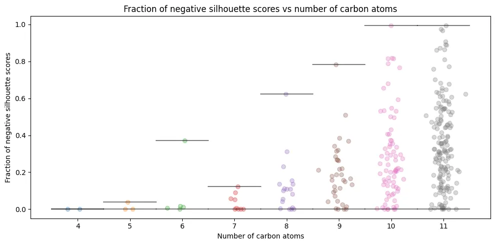
The individual analysis reveals dramatic variation:
- $C_{4}H_{10}$: Perfect clustering (0% misclassification), confirming our earlier 2D separation plots
- $C_{5}H_{12}$ to $C_{6}H_{14}$: Modest problems (1-8% misclassification rates)
- $C_{11}H_{24}$: Average 35% conformations misclassified per isomer
Some isomers experience up to 99.5% conformation misclassification (they become essentially unrecognizable in eigenvalue space). This directly connects to our earlier observation: mathematical representations that appear elegant may lack the structural nuances needed for practical discrimination.
Supervised Learning: Finding Hidden Structure
Both clustering metrics deliver the same conclusion: Coulomb matrix eigenvalues alone struggle to reliably distinguish constitutional isomers for larger alkanes. The mathematical elegance of eigenvalues encounters practical limitations as molecular complexity increases.
Supervised learning offers an alternative approach. Providing labels allows models to extract hidden patterns that elude clustering algorithms. The mathematical structure often requires explicit guidance for discovery.
I’ll focus on two baseline approaches: k-nearest neighbors and logistic regression. These represent fundamentally different learning paradigms (one memorizes patterns, the other learns linear boundaries) giving us insight into what types of structure might exist in eigenvalue space.
k-Nearest Neighbors: Pattern Recognition Through Memory
k-NN represents the simplest supervised learning approach: it stores all training examples and classifies new samples based on their closest neighbors. If eigenvalue patterns truly distinguish isomers, nearby points in eigenvalue space should belong to the same class.
This directly tests the local structure. Local neighborhoods often preserve meaningful distinctions even when global structure appears diffuse.
Testing Different Feature Representations
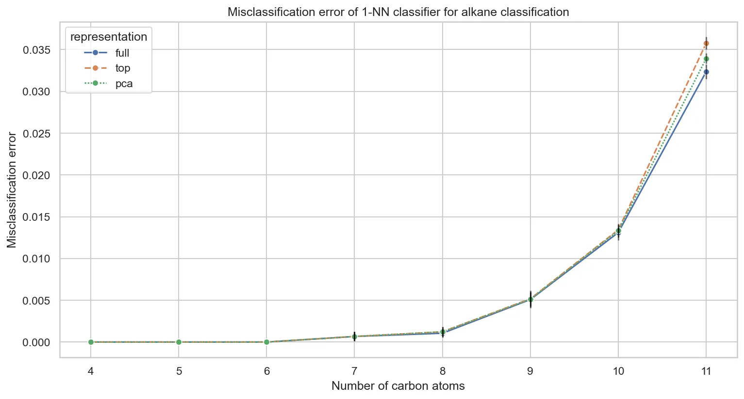
We compare three approaches: full eigenvalue vectors, top 10 eigenvalues only, and PCA-reduced representations.
Testing 1-nearest neighbor with full dimensionality:
from sklearn.model_selection import cross_val_score, StratifiedKFold
from sklearn.neighbors import KNeighborsClassifier

df_1nn = []

for n in range(4, 12):

    # Prepare the data for CnH2n+2
    X, y = prep_data(n=n)

    # Create knn classifier
    knn = KNeighborsClassifier(n_neighbors=1)

    # Set up stratified 5-fold cross-validation
    cv = StratifiedKFold(n_splits=5)

    # Perform cross-validation. Since 'cross_val_score' computes accuracy, we compute misclassification rate by subtracting accuracy from 1.
    acc_scores = cross_val_score(knn, X, y, cv=cv, scoring='accuracy')

    # Convert accuracy scores to misclassification error rates
    misclassification_error_rates = 1 - acc_scores

    # Calculate the average and standard deviation of the misclassification error rates
    avg_misclassification_error = np.mean(misclassification_error_rates)
    std_misclassification_error = np.std(misclassification_error_rates)

    print(f'C{n}H{2*n + 2}: {avg_misclassification_error:.2%} ± {std_misclassification_error:.2%}')

    df_1nn.append({
        'molecule': f'C{n}H{2*n + 2}',
        'avg_misclassification_error': avg_misclassification_error,
        'std_misclassification_error': std_misclassification_error,
        'n': n,
        'representation': 'full',
        'model': '1nn',
    })
The results are remarkable compared to unsupervised clustering:
C4H10: 0.00% ± 0.00%
C5H12: 0.00% ± 0.00%
C6H14: 0.00% ± 0.00%
C7H16: 0.07% ± 0.05%
C8H18: 0.11% ± 0.05%
C9H20: 0.51% ± 0.09%
C10H22: 1.31% ± 0.09%
C11H24: 3.24% ± 0.09%
Perfect classification for molecules up to $C_{6}H_{14}$, with remarkably low error rates even for complex molecules like $C_{11}H_{24}$. This dramatically improves over clustering, where 97% of $C_{11}H_{24}$ isomers had misclassified conformations.
Note on feature scaling: Standardizing features significantly degraded performance; eigenvalue magnitudes carry crucial structural information.
Comparing performance across different feature representations:
Key insights:
- Representation choice matters little for 1-NN. Full, top-10, and PCA representations perform nearly identically
- PCA slightly outperforms top-10 eigenvalues for larger molecules, capturing more structural variance
- Perfect classification persists through $C_{6}H_{14}$ regardless of representation
This confirms that discriminative information concentrates in the largest eigenvalues, validating our earlier PCA findings.
The Neighbor Count Effect
Testing k-NN with different neighbor counts (k=1, 3, 5) reveals a counterintuitive pattern:
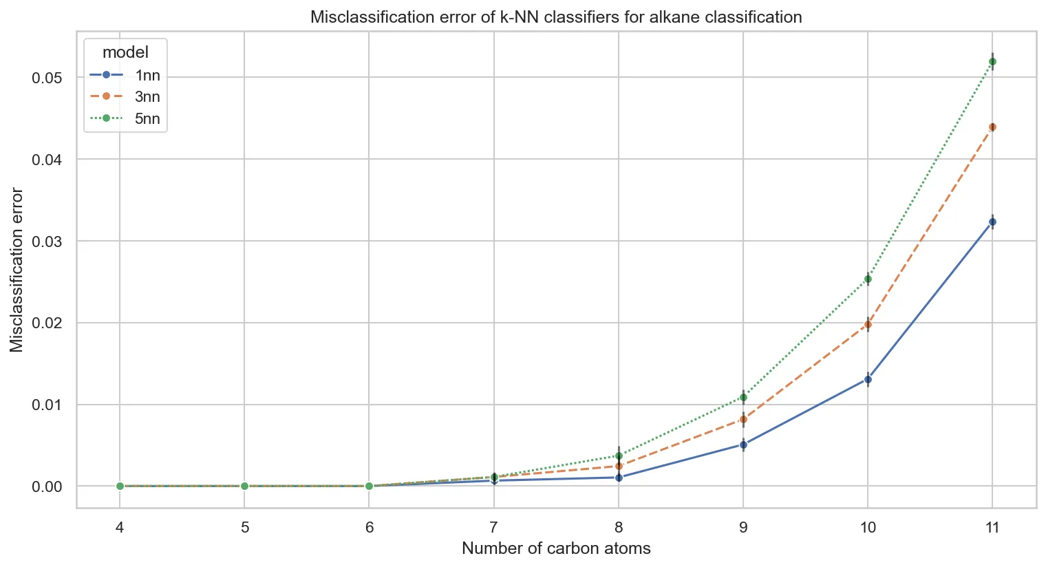
Why does performance degrade with more neighbors? This connects directly to our earlier clustering analysis. The eigenvalue space lacks meaningful local structure. When k-NN examines beyond the immediate nearest neighbor, it increasingly finds examples from different classes.
This validates our unsupervised findings: in the absence of clear cluster boundaries, examining more neighbors introduces noise.
Logistic Regression: Learning Linear Decision Boundaries
Logistic regression represents a fundamentally different approach. Logistic regression learns linear decision boundaries in eigenvalue space. If eigenvalues encode structural information linearly, this should work well.
We’ll focus on PCA-reduced representations to keep computation manageable, using insights from the k-NN analysis.
from sklearn.linear_model import LogisticRegression
from sklearn.pipeline import Pipeline
from sklearn.decomposition import PCA

df_lr = []

for n in range(4, 12):
    # Prepare the data for CnH2n+2
    X, y = prep_data(n=n)

    # Create logistic regression classifier with PCA
    lr = Pipeline([
        ('pca', PCA(n_components=10)),
        ('lr', LogisticRegression(
            max_iter=10_000,
            penalty='l2',
            solver='lbfgs',
            C=10.0,  # Reduced regularization
            random_state=42,
            n_jobs=-1,
        ))
    ])

    # 5-fold stratified cross-validation
    cv = StratifiedKFold(n_splits=5)
    acc_scores = cross_val_score(lr, X, y, cv=cv, scoring='accuracy')

    # Convert to misclassification rates
    avg_error = np.mean(1 - acc_scores)
    std_error = np.std(1 - acc_scores)

    print(f'C{n}H{2*n + 2}: {avg_error:.2%} ± {std_error:.2%}')
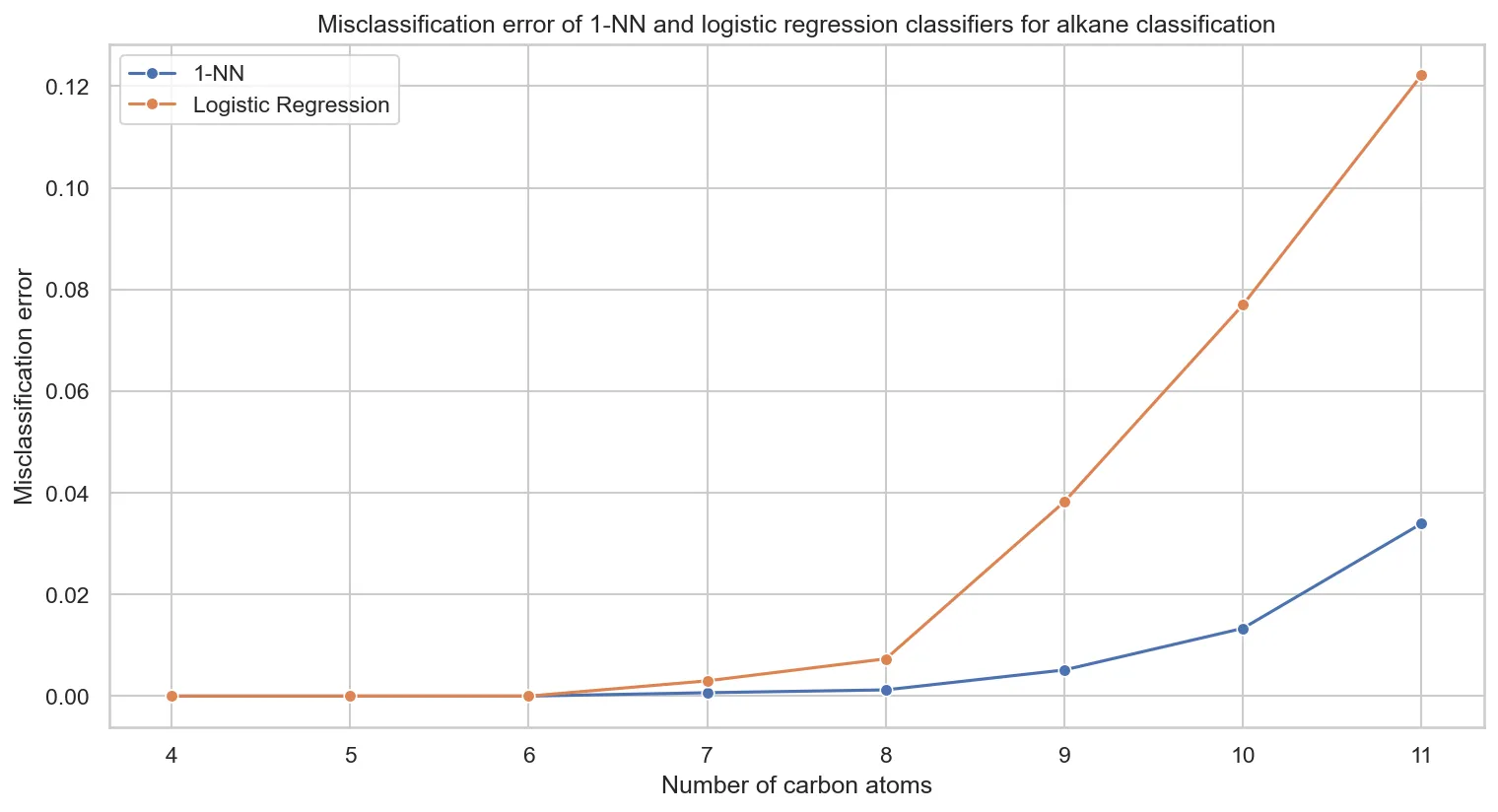
Comparing k-NN versus logistic regression performance:
Key observations:
- k-NN dominates across all molecular sizes
- Linear boundaries fail for larger molecules. This suggests nonlinear eigenvalue relationships.
- Performance gap grows with molecular complexity, indicating increasingly nonlinear structural patterns
Logistic regression’s performance indicates that discriminative patterns in eigenvalue space are fundamentally nonlinear. Capturing these complex relationships requires memory-based or non-linear approaches.
Implications for Molecular Representation
Our supervised learning experiments reveal a nuanced picture of Coulomb matrix eigenvalues as molecular descriptors. Eigenvalues preserve sufficient local structure for nearest-neighbor classification to work remarkably well, despite lacking clean global clusters.
This analysis reveals important lessons about molecular representations:
- Practical utility requires robust empirical performance alongside mathematical elegance: Mathematical elegance often accompanies fundamental limitations in complex spaces.
- Context matters: Representations exhibit distinct performance characteristics under supervised versus unsupervised conditions.
- Molecular complexity is challenging: Even simple alkanes test our best descriptors.
- Local vs. global structure: Local neighborhood structures often contain highly discriminative information.
For practitioners working with molecular representations, it is crucial to test multiple learning paradigms. Supervised and unsupervised approaches often yield different insights. Furthermore, logistic regression’s poor performance indicates that discriminative patterns in eigenvalue space are fundamentally nonlinear. Capturing these complex relationships requires memory-based or non-linear approaches.
Real-World Impact: Why does this matter beyond an academic exercise? Robust molecular representations are the engine driving modern computational chemistry. Whether we are accelerating drug discovery pipelines, designing novel materials, or running large-scale molecular dynamics simulations, the quality of our underlying representations dictates the success of our machine learning models. Understanding exactly where and why simpler descriptors like Coulomb matrix eigenvalues fail helps us design the next generation of graph neural networks and transformer-based architectures that power today’s scientific breakthroughs.
The data pipeline that generated the datasets used in this analysis is available at the Synthetic Isomer Data Generation Pipeline project page.
