The MIST paper makes a claim I wanted to test from an angle its authors did not take. They show that their model’s embedding space organizes chemical concepts along physically meaningful directions. Lipinski’s Rule of Five is linearly decodable from frozen activations. Unsupervised projections of the embeddings separate aromatic from anti-aromatic compounds along Hückel’s rule, and none of that was labelled during training.
All of that structure is derived from a SMILES string.
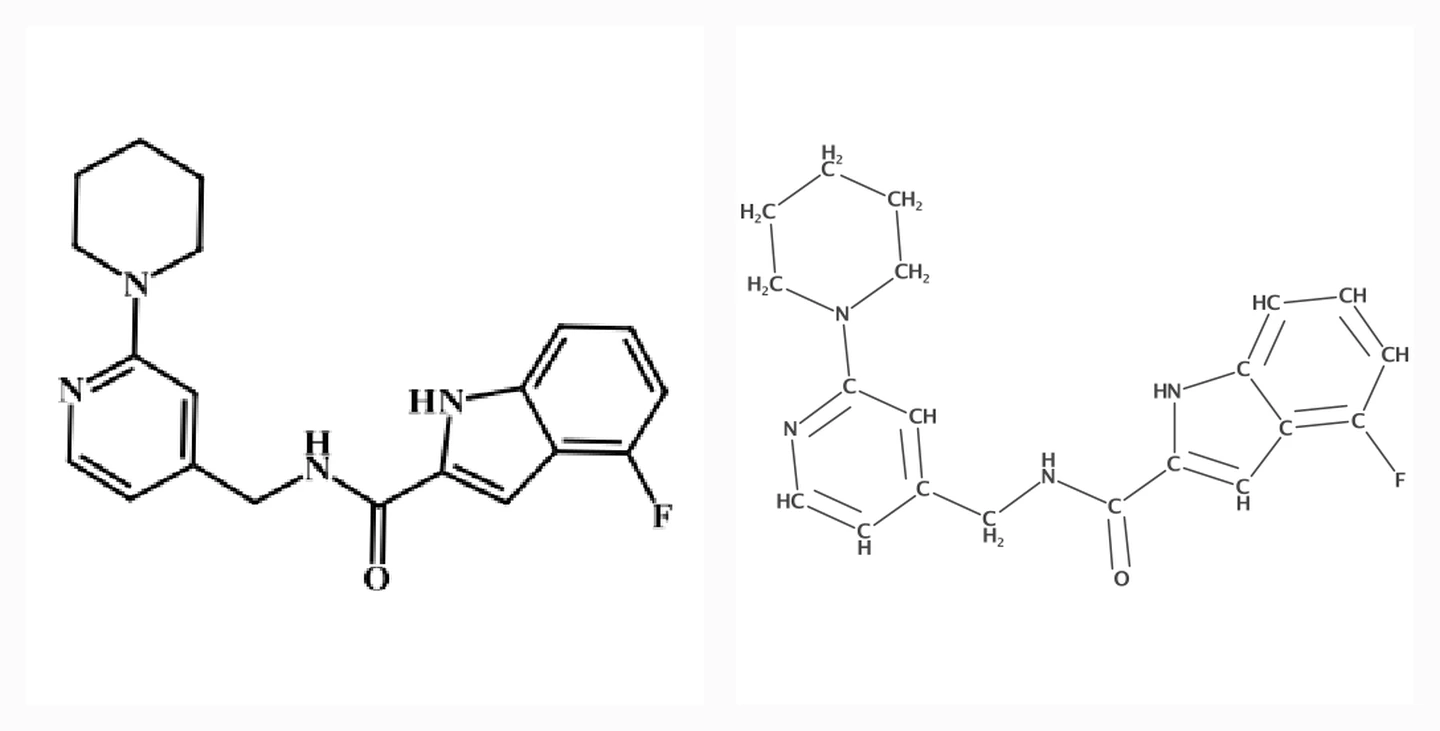
Molecules are also drawn. A structure diagram carries the same topology a chemist reads directly off the page, in a form no language model ever sees. So I wanted to know whether MIST’s geometry is reachable from pixels, or whether it is a property of the string.
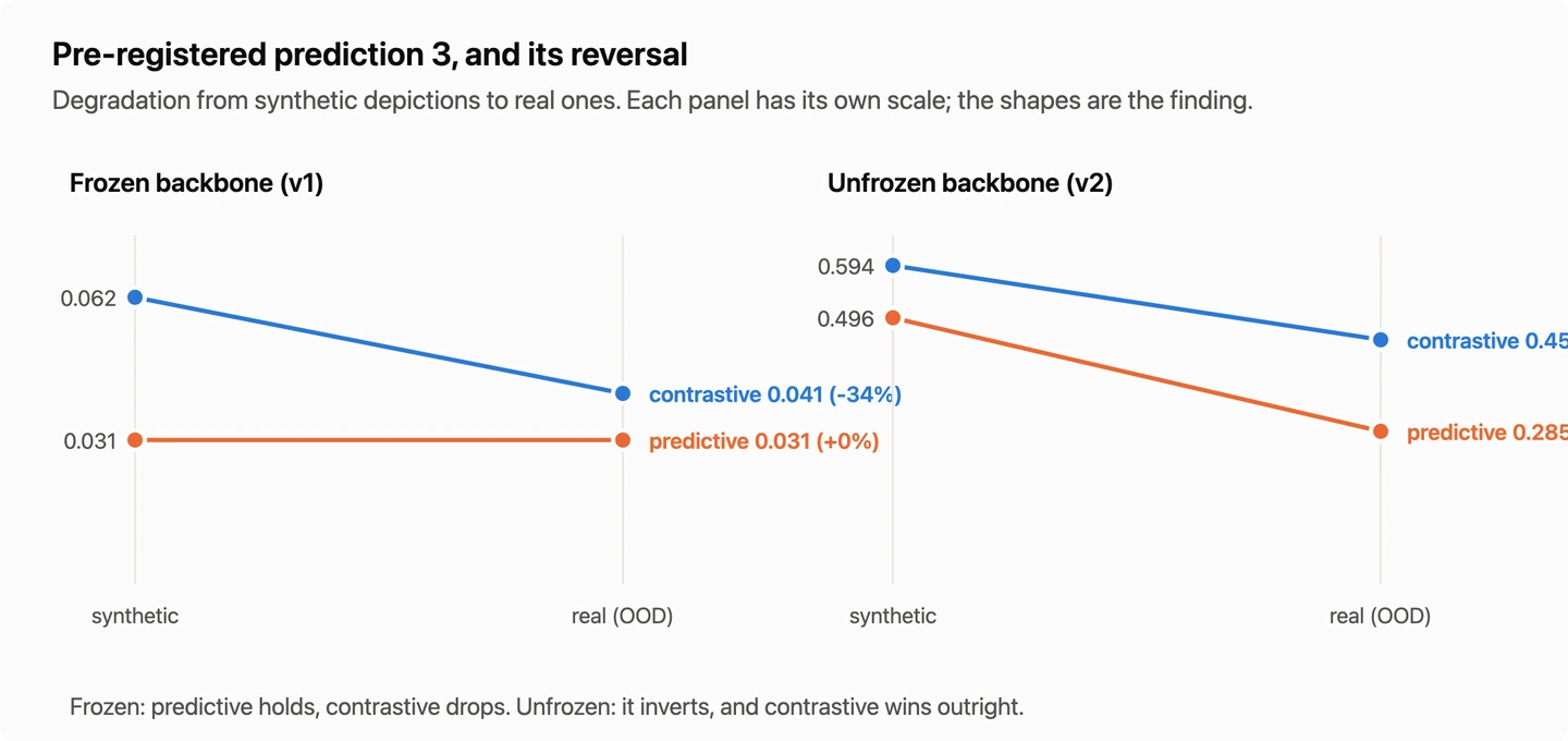
There are two standard ways to teach one model to land where another one does. You can push negatives apart with a contrastive loss, or you can skip the negatives and regress the target directly. I expected the predictive one to transfer better to real drawings, because a contrastive objective can exploit shortcuts that only exist inside a training batch. I wrote that down before running anything.
It held, then it reversed, and the mechanism I had named for it was wrong in both cases.
What I Built
One vision tower, one frozen text tower, and a single linear map between them.
| Vision tower | DINOv2 ViT-S/14 with registers, 21,629,952 parameters, 384-d output |
| Text tower | MIST-28M, frozen throughout, pooled last_hidden_state[:, 0, :], 512-d output |
| Head | one linear map, 384 to 512, 197,120 parameters |
| Training data | 1M PubChem molecules, about 2M RanDepict depictions at 224px |
| Schedule | 24 epochs, batch 256 |
Arm A optimizes the SigLIP sigmoid pairwise loss. Arm B regresses the frozen target in latent space with a smooth-L1 loss and no negatives, which is the I-JEPA move applied as an alignment head rather than as pretraining. Everything else is held identical: same molecules, same splits, same seed, same schedule, same evaluation, checked by an assertion before any table prints. Every number below is one seed.
Two details in the setup are load-bearing.
The pooling is MIST’s own. Their embedding is the last-layer hidden state at the first token, so anything else measures a different space. Loading the checkpoint with AutoModel also attaches a randomly initialized pooler unless you ask it not to, and pooler_output from that pooler returns plausible noise.
The contrastive labels come from molecular identity rather than batch position. Two rows in a batch can be depictions of the same molecule, and treating them as negatives because they sit at different indices would penalize the model for being right. That detail matters more than it looks, and I will come back to it.
This is not an OCSR contribution. Reading a molecule out of a picture is a mature field, and MolScribe, MolGrapher, DECIMER and Img2Mol all do it well. What is here is a controlled experiment about alignment objectives that happens to run on a domain with a real evaluation surface.
That domain has a catch worth stating early, because it shapes which number is the result. The training depictions are rendered from SMILES strings. A picture drawn from a string carries no information the string did not already have, so the in-distribution task is closer to inverting a renderer than to reading chemistry. Transfer to depictions that came from the world is the part that tests something. That is why the out-of-distribution slice is the headline and the in-distribution number is context.
I came to MIST from the tokenizer side. I had published a controlled comparison of BPE and Unigram-LM over chemistry SMILES a few weeks earlier, and MIST is a SMILES foundation model whose headline contribution is its own tokenizer. I was reading the paper closely for that reason and stayed for the embedding geometry.
What I Registered In Advance
Three predictions, committed before any training run existed:
- Both arms will be near-ceiling on in-distribution synthetic retrieval, and that number on its own will mean almost nothing.
- The arms will separate, if at all, on the WildMol-10k OOD slice and the scaffold-split linear probe. That gap is the result.
- Arm B is expected to hold up better OOD, on the reasoning that regressing a fixed target cannot exploit in-batch shortcuts the way a contrastive objective can. This is a guess and is written down so it can be wrong in public.
I also registered what would count as a clean negative and ship as the result: both arms at or near chance on the OOD slice and the probe, with all baselines behaving correctly. That sentence turns out to matter more than the predictions do.
What Had To Pass First
Four gates run before any headline number is believed, because a comparison between two arms says nothing if the harness scoring both of them is broken.
| gate | result | what it rules out |
|---|---|---|
| oracle retrieval, a perfect predictor | R@1 = 1.0 | the retrieval harness itself |
| MIST against Tanimoto similarity | r = +0.42 | a target that carries no chemistry |
| random-embedding control | +0.0014 centered cosine | a metric that leaks |
| trivial image-statistics floor | +0.0924 centered cosine | mistaking ink for structure |
The image-statistics floor is the one that earns its keep below. It is what a model scores using nothing but coarse pixel statistics, and any headline has to clear it.
A Perfect Model Scored Zero
Raw cosine against MIST measures almost nothing. Its embeddings occupy a narrow cone, where two unrelated molecules sit at cosine 0.517 and a model that ignores its input entirely and emits the training centroid scores 0.720. So every cosine in this project is centered, and each side is centered by its own training-split mean:
$$ \mathrm{cc} = \cos\left(\hat{\mathbf{u}} - \bar{\hat{\mathbf{u}}}_{\text{train}},\ \mathbf{y} - \bar{\mathbf{y}}_{\text{train}}\right) $$
Chance is zero. Both centroids come from the training split, since centering a held-out set by its own mean leaks that set’s geometry into its own score.
The version I shipped first subtracted the target centroid from both sides. That is valid only while the prediction sits at roughly the target’s scale. Arm B’s smooth-L1 pins it there. Arm A’s loss L2-normalizes both sides internally, so it constrains the output norm not at all, and weight decay shrinks it with nothing opposing.
Take an oracle predictor $\hat{\mathbf{u}} = s\mathbf{y}$, whose true cosine is exactly 1 for every $s > 0$:
| $s$ | $\lVert\hat{\mathbf{u}}\rVert$ | centered by target | centered by own mean |
|---|---|---|---|
| 1.00 | 22.28 | +1.0000 | +0.9999 |
| 0.50 | 11.14 | +0.6100 | +0.9999 |
| 0.10 | 2.23 | +0.0453 | +0.9999 |
| 0.045 | 1.00 | -0.0103 | +0.9999 |
A perfect model emitting unit-norm vectors scored below chance.
On the real 20K run, that defect scored a working contrastive model at +0.1088, inside noise of the +0.1058 image-statistics floor. Arm A’s head was emitting norm 6.35 against MIST’s 22.28. Under the corrected metric the same checkpoint scores +0.3052.
The uncomfortable part is what that number was. I had registered, in advance, that both arms landing at the floor with every baseline behaving correctly would be a clean negative and would ship as the result. The defect produced precisely that. Every exit criterion passed.
No test caught it. What caught it was asking what a perfect model would score under this metric, which is a question whose answer is knowable before you ask it.
Registering a prediction stops the goalposts moving once data exists. It does nothing at all about a defect that happens to confirm the prediction, and it makes that case more expensive rather than less, because the incentive to accept a number and stop looking is strongest exactly where you said the number would be.
There was a second defect of the same shape waiting. Had the contrastive labels come from batch position instead of molecular identity, the model would have been penalized for putting two depictions of one molecule in the same place. That depresses contrastive transfer and leaves predictive untouched, because only the contrastive loss reads other rows in the batch, which is prediction 3 arriving as an artifact of the label matrix.
The Data Ran Out
With the backbone frozen, I fitted a log-linear law to the closed-form ridge ceiling over 1K to 16K molecules. It described that range well, at r = 0.9906. Extrapolated, it said 1M molecules would reach +0.600.
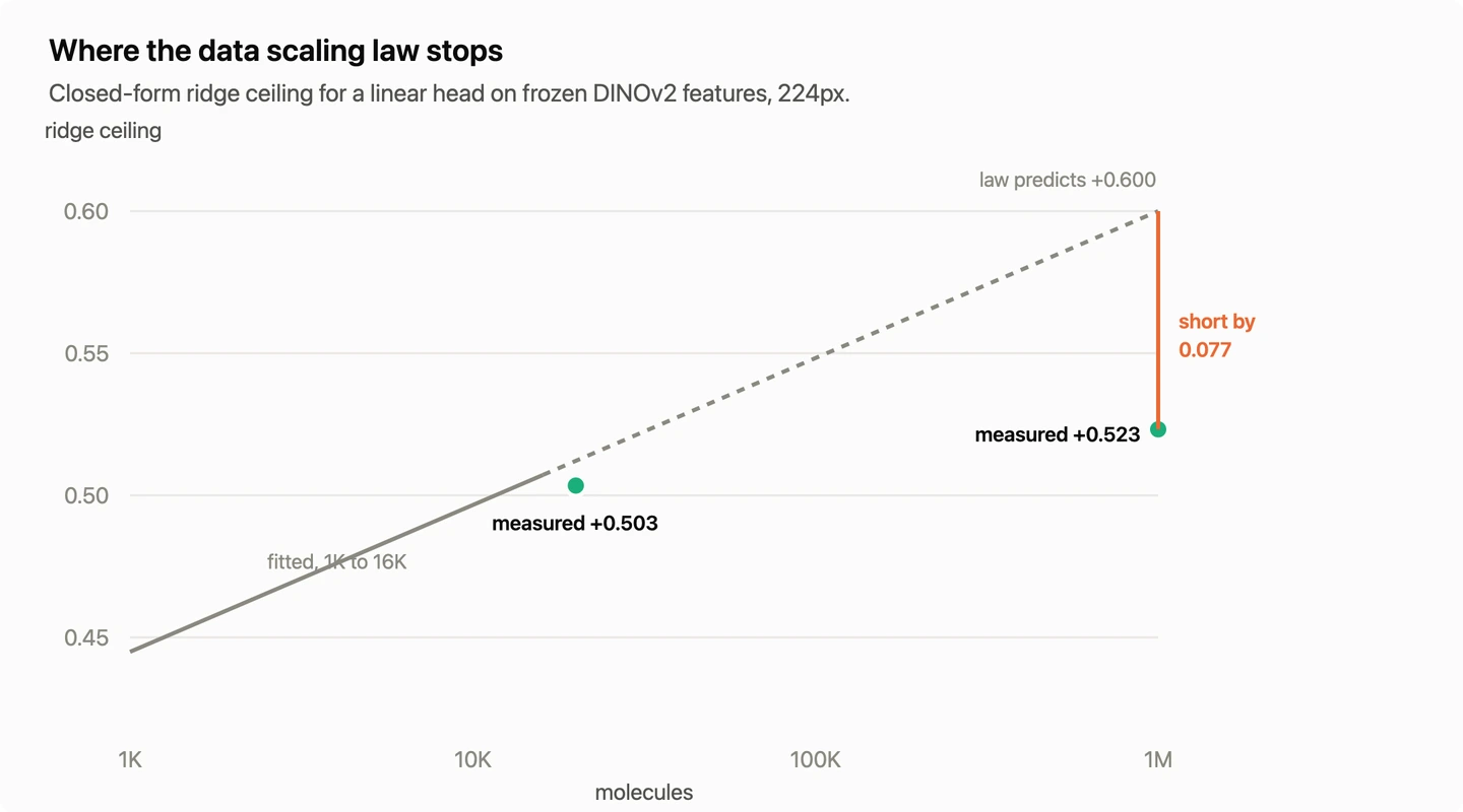
Going from 796K to 1.6M depictions bought +0.0002.
The mechanism is in the features rather than the sample. On these images, 54.3% of DINOv2’s feature variance is depiction style rather than molecular identity. Two renders of the same molecule sit at cosine 0.857, and two different molecules sit at 0.809, which leaves very little room between “same structure” and “different structure” for a linear head to work with.
A linear head can reorganize what the backbone encodes. It cannot manufacture what the backbone discarded. That showed up directly in the probes, where alignment helped on the tasks whose property the frozen features already carried and did nothing at all on three of seven.
This is the second prediction I made in advance and missed, and it was the more expensive one, because I had been about to spend on data.
Unfreezing Reversed My Own Prediction
Letting the backbone move changes the picture. I swept two trainable modes rather than picking one: LoRA at rank 16 on the attention projections of all twelve blocks, and the top four blocks plus the final norm. The top-blocks mode won on every layer, and LoRA was also 1.84x slower per step despite training 16x fewer parameters, because backward cost tracks how deep the pass goes rather than how many parameters update.
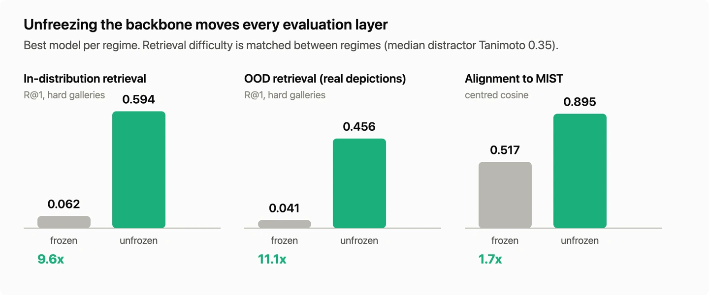
The out-of-distribution gate is what makes this mean something, and it matters because an earlier lever failed it. Running the backbone at its native 518px instead of 224 improved every synthetic-image metric, several by multiple standard deviations, and moved the real-depiction metric by less than one. That lever was fitting RanDepict’s particular ink rather than learning chemistry. Unfreezing does not behave that way.
Then the registered prediction inverted.

The ordering was a property of the frozen bottleneck rather than of the objectives. Give the contrastive objective a backbone it can actually shape and it is the one that degrades less.
Had I only run the frozen half, I would have published a confirmed prediction with a mechanism attached, and the mechanism would have been wrong. The number was fine. The explanation underneath it was not, and nothing in the frozen regime could have told me.
Prediction 1 was wrong outright, which is worth recording since I registered it as the boring one. I expected in-distribution retrieval to sit near ceiling and carry no information. It came in at 0.0617 and 0.0310 against a 0.0156 chance floor, which is why it is reported throughout rather than waved off.
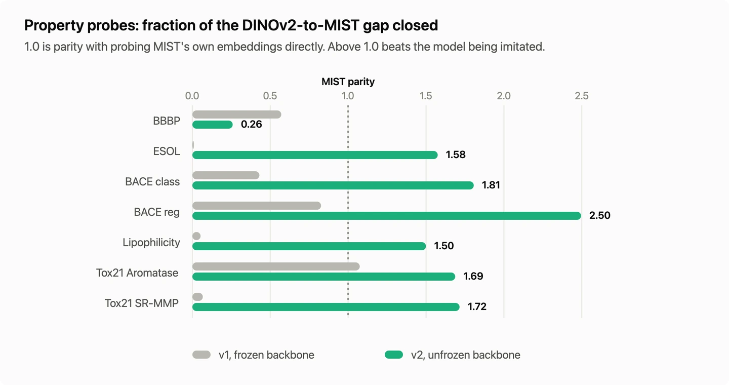
On one fixed checkpoint, the aligned image embedding out-probes MIST-direct on 6 of 7 tasks, losing only BBBP. Best-of-eight beats it on 7 of 7, and I am not quoting that as the result because it is selection over eight tries. The honest reading is that MIST bounds MIST-reconstruction rather than every downstream task where vision carries independent signal.
The Fairest Rule Picked the Worst Checkpoint
The two arms have losses on different scales, so selecting each on its own loss would compare two selection procedures rather than two objectives. I selected on centered cosine instead, the one metric both arms are measured by. Neutral by construction.
It chose epoch 1 of 24 for the contrastive arm, in both trainable modes.
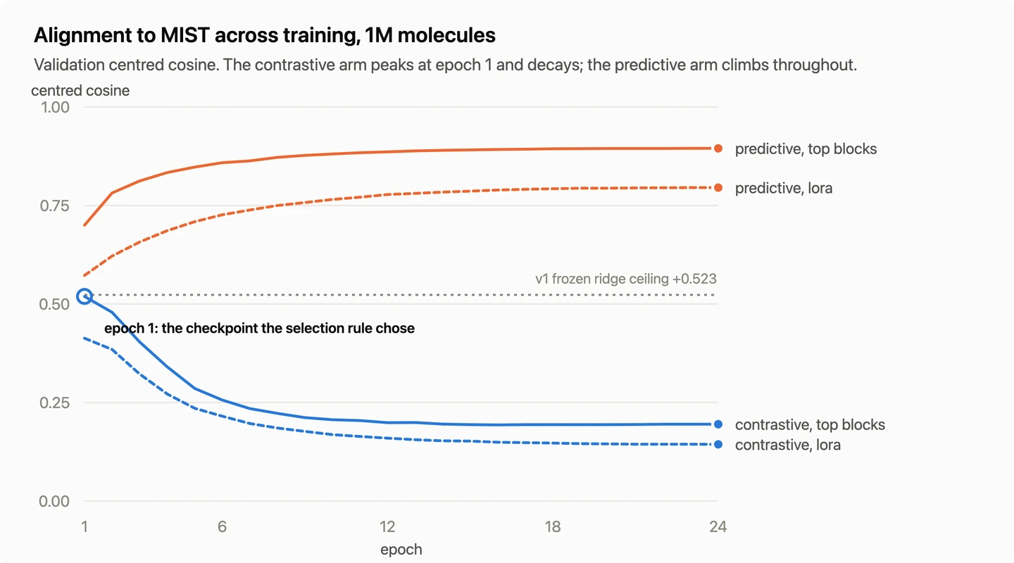
I had written this down on the first day of the project, at the milestone where the two arms first ran side by side:
Selecting on it hands Arm A its worst retrieval checkpoint. Selecting on retrieval instead would reverse the ranking and would be equally defensible and equally partial.
And in the same entry, on why I was recording it at all:
Recording it now, at M3, because it is exactly the kind of thing that gets quietly resolved in whichever direction the first table happened to point.
I scoped that observation as measured outside the contrastive arm’s viable regime, which was correct at the time. At 20K molecules there is no batch size that is both a real contrastive batch and a small fraction of the dataset, so the arm was running at 256 while SigLIP’s own calibration assumes 16,384. Rebuilding at 1M fixed that, and the failure happened anyway, in the regime where it counted.
The obvious objection is that the constraint itself was the cause. Holding the learning rate, the schedule and the checkpoint rule identical across two objectives that optimize different things does not make a comparison fair, it handicaps whichever arm does not match the shared choice.
The repair would be to let each arm carry its own schedule, and gradient accumulation is the specific one that was on the table. I did not add it, and I still think that was right. Accumulation enlarges the contrastive arm’s negative pool and does nothing for the predictive one, so adding it converts a comparison of objectives into a comparison of training budgets. That is a second bias rather than a smaller one.
What I did not do was change the rule after seeing what it cost. Retrofitting a selection criterion once results exist is the specific thing pre-registration exists to prevent, so both epochs are reported instead.
Three shared choices ended up bending against the contrastive arm, all in the same direction. Weight decay at 0.05 against a scale-invariant loss, which is what produced the metric defect. Batch 256 against a calibration assuming 16,384. A selection metric that measures direction agreement, which is close to what the predictive arm optimizes directly.
It won the layer I had named in advance as the deciding one anyway, 0.4555 against 0.2847. So the measured gap is a floor rather than an estimate.
What I Would Not Trust Here
Three things would change a conclusion above, in order of how much.
The probe splits shift in composition. ESOL’s training split is 35% acyclic molecules against 0% of validation and test, and Tox21 is about 32%. Acyclic molecules have no Bemis-Murcko scaffold, so a scaffold split places them all in one group and that group is large enough to land in train. ESOL is the largest probe gain in this post, and it was scored on a held-out set with none of the molecules that make up a third of what it trained on.
One seed, and the sigmas are uneven. The only repeats in the project are a 5-seed frozen sweep at 20K. Arm A retrieval sigma runs .002 to .005 and BBBP .004 to .011. The retrieval orderings clear that by roughly two orders of magnitude and are safe. Individual probe cells do not clear it, and several rows show test scores above validation, which is what noise on a small scaffold-split test set looks like.
The predictive arm was truncated. It was still rising at epoch 24 in both modes, and 24 epochs was inherited from the frozen regime where it was enough. Its numbers are a lower bound, which cuts against this post’s own conclusion.
Conclusion: One Number Cannot Rank Two Objectives
The comparison never resolved to a winner in the way I expected when I started, and the reason is more interesting than a winner would have been. Under a frozen backbone the predictive arm holds up better, and that ordering is a fact about the bottleneck. Under a trainable one the contrastive arm wins out of distribution, and it does so while carrying every shared-procedure handicap.
Three of the four things above were numbers I initially believed. A metric that scored a perfect model below chance, a scaling law that was accurate everywhere I had fitted it, and a selection rule that was neutral by construction. Each looked fine, and each was checkable in advance by asking what a known answer should be.
The one that still bothers me is the metric, because it produced the exact result I had written down as shippable. Pre-registration protected me from moving the goalposts and did nothing about that.
Code, weights and data are public. The repository carries the full results, the harness gates and the pre-registration verbatim. The two aligned models are on Hugging Face as contrastive and predictive, and the 20K depiction set is published so the comparison can be re-run without standing up the rendering environment.