Introduction
Understanding how individual atoms move on crystal surfaces is fundamental to materials science, catalysis, and nanotechnology. This atomic-scale motion, called adatom diffusion, drives processes like thin film growth and surface chemical reactions.
While learning molecular dynamics simulations for my graduate work, I discovered these simulations generate valuable training data for machine learning models. This tutorial walks through simulating copper adatom diffusion on a Cu(100) surface using LAMMPS, building on Eric N. Hahn’s excellent adatom tutorial.
What you’ll learn:
- Setting up LAMMPS for surface diffusion simulations
- Understanding simulation parameters and their impact
- Visualizing results with Ovito
- Analyzing trajectory data for ML applications
- Connecting simulation data to machine learning workflows
In this tutorial, we will explore both Copper (Cu) and Platinum (Pt) to show how atomic properties affect diffusion behavior, providing valuable insights for training element-aware ML models.
Prerequisites
Before starting this tutorial, you’ll need:
- LAMMPS with EAM potential support (version 2020 or later recommended)
- Python 3.x with matplotlib for analysis scripts
- Ovito (free version) for trajectory visualization
- Cu01.eam.alloy potential file from the NIST repository
- Basic familiarity with molecular dynamics concepts (atoms, forces, timesteps)
Understanding Adatoms and Surface Diffusion
What is an Adatom?
An adatom (adsorbed atom) sits on a crystal surface but isn’t incorporated into the bulk structure. Adatoms have fewer bonds than fully coordinated bulk atoms, making them highly mobile and reactive.

Why Study Adatom Diffusion?
Adatom diffusion is important for several technological processes:
- Thin film growth: Adatoms are the building blocks of deposited films
- Catalysis: Many reactions happen at these mobile surface atoms
- Corrosion: How surface atoms move affects material degradation
- Self-assembly: Adatom movement enables formation of ordered structures
From a machine learning perspective, adatom diffusion is an ideal test case because:
- Well-understood physics provides ground truth for validation
- Small system size enables extensive simulation
- Behavior varies significantly with temperature and atomic species
- Systematic data generation across different conditions
Why Cu(100)?
Cu(100) surfaces are well-studied in literature, making them excellent benchmarks. The face-centered cubic (fcc) structure creates clear diffusion pathways, and copper’s moderate binding energy lets us observe diffusion at reasonable temperatures without extreme computational demands.
Simulation Overview
Before diving into the code details, let’s understand the simulation design:
Key Simulation Parameters
| Parameter | Value | Why this choice |
|---|---|---|
| System size | $8 \x8 \x6$ unit cells | Large enough to avoid edge effects while keeping simulation time reasonable |
| Ensemble | NVT (constant volume, temperature) | Appropriate for surface studies where pressure isn’t the focus |
| Potential | EAM (Embedded Atom Method) | Captures metallic bonding better than simple pair potentials |
| Time step | 5 fs | Small enough for numerical stability while allowing reasonable run times |
| Duration | 500 ps | Long enough to see multiple diffusion events |
| Temperature | 600 K (bulk), 850 K (surface) | Creates thermal gradient that drives surface motion |
Simulation Strategy
The approach uses a thermal gradient setup:
- Bottom layers: Fixed to represent bulk crystal
- Middle layers: Heated to 850 K for thermal energy
- Top layers and adatom: Equilibrate to $\sim 600$ K for diffusion
- This mimics real heat flow from substrate to surface
The complete LAMMPS script implementing this approach:
### Original Created by Eric N. Hahn  ###
### [email protected] ###

### Modifications by Hunter Heidenreich, CSE lab (Harvard, 2023)
### [email protected]
### 2023-09-01

### Simulating adatoms ###
### Version 0.2 ###


units metal
dimension 3
boundary p p s
atom_style atomic

lattice fcc 3.614
variable cubel equal 4
variable fixer1 equal "v_cubel+2"
variable fixer2 equal "v_cubel+1.49"
region  box block -${cubel} ${cubel} -${cubel} ${cubel} -${fixer1} 1 units lattice
region cbox block -${cubel} ${cubel} -${cubel} ${cubel} -${fixer1} 0 units lattice
create_box 1 box
create_atoms 1 region cbox
create_atoms 1 single -0.5 0 0.5 units lattice
region hold block INF INF INF INF -${fixer1} -${fixer2} units lattice
region temp block INF INF INF INF -${fixer2} -${cubel} units lattice
group hold region hold
group temp region temp

pair_style eam/alloy
pair_coeff * * Cu01.eam.alloy Cu

timestep        0.005
compute         new all temp
velocity        temp create 600 12345
fix heater temp temp/rescale 1 850 850 5 1
fix nve all nve
fix freeze hold setforce 0 0 0

variable e     equal pe
variable k     equal ke
variable t     equal etotal
variable T     equal temp
fix energy all ave/time 1 50 50 v_k v_e v_t v_T file energy_avg.txt

minimize 1.0e-4 1.0e-6 1000 10000

dump eve all custom 5 dump.lammpstrj id type xu yu zu   # fx fy fz  # uncomment for forces
dump_modify eve sort id

thermo 50
run 100000  # 100_000 * 5 fs = 500 ps
Line-by-Line Breakdown
Let’s examine each part of the LAMMPS script:
Simulation Setup
Units
units metal
Sets simulation units to “metal” units (a standard choice for metallic systems). Key conversions: length in $\text{\AA}$, energy in eV, time in ps. Full details in the LAMMPS documentation.
dimension 3
Sets 3D simulation.
boundary p p s
Boundary conditions: periodic in x,y (infinite surface) and shrink-wrapped in z (finite surface height). This allows the adatom to potentially leave the surface if needed.
atom_style atomic
Uses “atomic” style, atoms as point masses without internal structure. Standard for metallic systems.
Lattice
lattice fcc 3.614
Defines face-centered cubic lattice with experimental Cu lattice constant ($3.614 \text{ \AA}$).
variable cubel equal 4
variable fixer1 equal "v_cubel+2"
variable fixer2 equal "v_cubel+1.49"
Define variables for simulation box dimensions. cubel=4 sets system size, while fixer1 and fixer2 define the frozen and heated regions.
region  box block -${cubel} ${cubel} -${cubel} ${cubel} -${fixer1} 1 units lattice
region cbox block -${cubel} ${cubel} -${cubel} ${cubel} -${fixer1} 0 units lattice
Define regions: box for the entire simulation volume and cbox for crystal creation (excludes the surface layer where we’ll place the adatom).
create_box 1 box
create_atoms 1 region cbox
create_atoms 1 single -0.5 0 0.5 units lattice
Create simulation box, populate with Cu atoms, then add single adatom at specified position.
region hold block INF INF INF INF -${fixer1} -${fixer2} units lattice
region temp block INF INF INF INF -${fixer2} -${cubel} units lattice
group hold region hold
group temp region temp
Define atom groups: hold (frozen bottom layers) and temp (heated middle layers for thermal energy).
pair_style eam/alloy
pair_coeff * * Cu01.eam.alloy Cu
Use Embedded Atom Method (EAM) potential for metallic bonding. The Cu01.eam.alloy potential from Mishin et al. is available from the NIST repository.
timestep 0.005
5 femtosecond timestep (small enough for numerical stability).
Initial Conditions
velocity temp create 600 12345
Initialize velocities for 600 K temperature using random seed 12345.
fix heater temp temp/rescale 1 850 850 5 1
fix nve all nve
fix freeze hold setforce 0 0 0
Three fixes control dynamics:
heater: Maintains 850 K in middle layersnve: Velocity Verlet integration for all atomsfreeze: Sets forces to zero for bottom atoms
variable e     equal pe
variable k     equal ke
variable t     equal etotal
variable T     equal temp
fix energy all ave/time 1 50 50 v_k v_e v_t v_T file energy_avg.txt
Track energies and temperature, averaging every 50 timesteps and writing to file.
Execution
Minimization
minimize 1.0e-4 1.0e-6 1000 10000
Relax initial structure. Should converge quickly, indicating the system is already well-optimized.
Output Setup
dump eve all custom 5 dump.lammpstrj id type xu yu zu   # fx fy fz  # uncomment for forces
dump_modify eve sort id
Write atomic positions every 5 timesteps, sorted by atom ID. Uncomment force components if needed for analysis.
Production Run
thermo 50
run 100000  # 100_000 * 5 fs = 500 ps
Run simulation for 500 ps with thermo output every 50 steps.
Visualization and Analysis
Visualize results using Ovito, a free atomistic visualization tool:
- Open the trajectory file in Ovito
- Color atoms by z-coordinate
- Restrict height range to $0\text{-}2 \text{ \AA}$ for surface focus
- Animate to observe diffusion events
Analysis Results
The simulation generates rich data for machine learning applications:
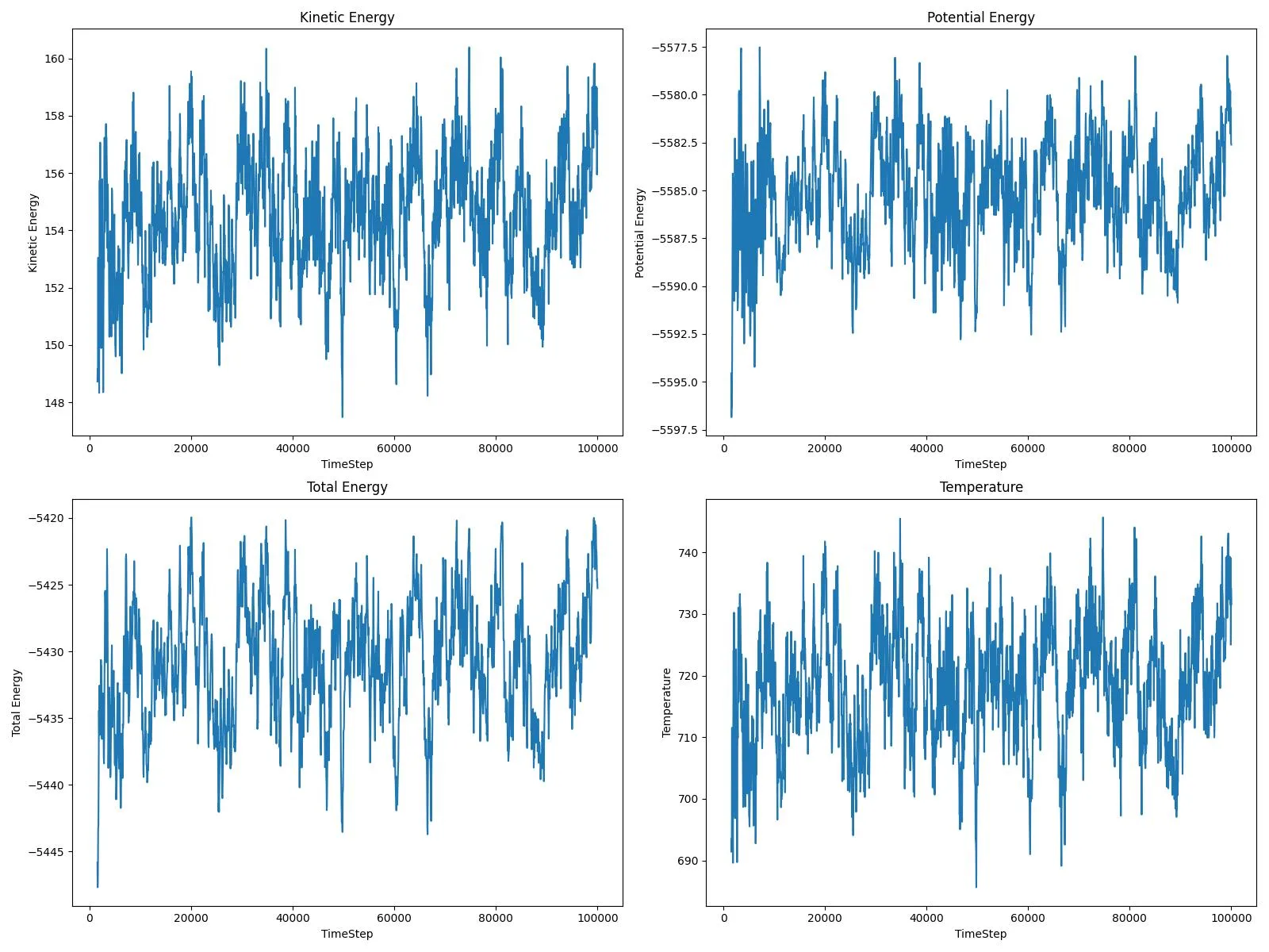
Energy Analysis
Energy fluctuations reveal thermal motion patterns:

Skipping initial equilibration (first 30 steps), these fluctuations enable:
- Anomaly detection: Identifying unusual diffusion events
- Temperature prediction: Estimating local temperature from atomic motion
- Stability analysis: Detecting equilibrium states
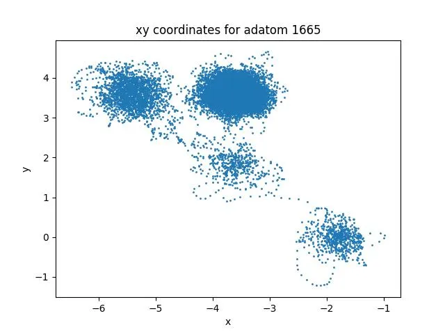
Trajectory Analysis
Adatom motion reveals diffusion mechanisms:

This data enables:
- Path prediction: Training models for future position forecasting
- Diffusion coefficient estimation: Learning temperature-mobility relationships
- Transition state identification: Detecting hops between stable sites

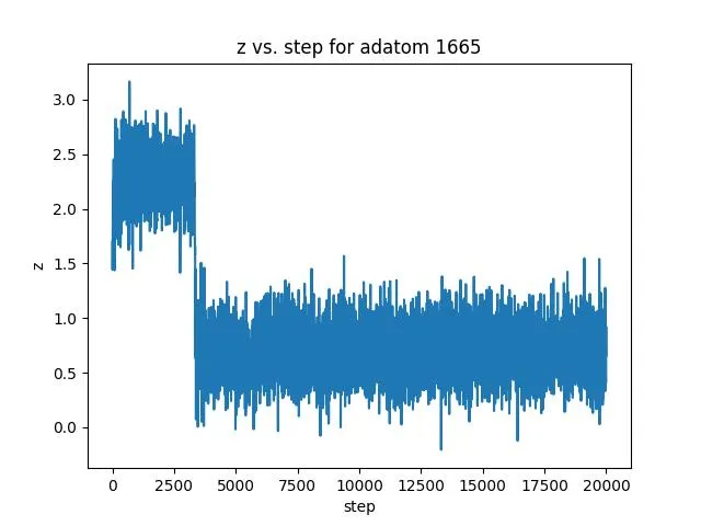
Z-coordinate data shows exchange events where the adatom swaps with surface atoms (crucial for surface chemistry understanding). This enables:
- Event classification: Distinguishing diffusion vs. exchange mechanisms
- Activation barrier estimation: Learning energy landscapes from fluctuations
- Surface coordination analysis: Correlating height with local environment
Machine Learning Applications
This simulation produces multiple data types for ML training:
- Coordinate trajectories: Neural network potential inputs or graph neural network features
- Energy time series: Regression model features for system property prediction
- Event annotations: Supervised learning labels for diffusion mechanism classification
- Environmental descriptors: Local atomic arrangement features
Systematic MD simulations generate large, labeled datasets across varied conditions.
Extending to Platinum: Mass and Bonding Effects
To understand how different elements behave, we can extend this framework to platinum (Pt). Platinum’s higher atomic mass and stronger metallic bonding create notably different diffusion behavior, providing valuable comparative data for machine learning.
Key Differences from Copper
| Parameter | Copper (Cu) | Platinum (Pt) | Impact |
|---|---|---|---|
| Atomic mass | 63.5 u | 195.1 u | Slower diffusion, longer correlation times |
| Lattice const. | 3.614 Å | 3.96 Å | Larger diffusion barriers, different pathways |
| Potential | Mishin et al. | Zhou et al. | Different interaction strengths |
| Melting point | 1358 K | 2041 K | Stronger surface binding |
Modifying the LAMMPS Script
The platinum simulation uses the exact same framework as the copper case, with three simple element-specific modifications:
- Lattice constant: Change
lattice fcc 3.614tolattice fcc 3.96 - Potential file: Change
Cu01.eam.alloytoPt_Zhou04.eam.alloy(available from the NIST repository) - Element specification: Change
CutoPtin thepair_coeffline
These simple changes capture the essential physics differences between elements while maintaining the same simulation protocol, which is ideal for generating comparative datasets for ML training.
Expected Behavior vs. Copper
When you run the analysis scripts on the platinum trajectory, you will observe:
- Slower motion: Heavier atoms move more slowly at the same temperature. Platinum’s ~3x greater mass reduces diffusion rates.
- Higher energy barriers: Stronger metallic bonding creates deeper potential wells, requiring more thermal energy for diffusion hops.
- Different pathways: The larger lattice constant changes the energy landscape, potentially favoring different diffusion mechanisms.
Comparing Cu and Pt trajectories enables training element-aware models that account for atomic mass effects, binding strengths, and temperature scaling across different metals.
Code and Data
The complete simulation scripts and analysis tools are available for reproducibility:
Energy Analysis Script
# Hunter Heidenreich, 2023
# Plots the energy of a simulation over time.

import matplotlib.pyplot as plt
from argparse import ArgumentParser

if __name__ == '__main__':
    parser = ArgumentParser()
    parser.add_argument('--input', type=str, required=True)
    parser.add_argument('--output', type=str, required=True)
    parser.add_argument('--skip', type=int, default=1)
    args = parser.parse_args()

    # Parse energy data
    data = {'ts': [], 'kes': [], 'pes': [], 'tes': [], 'Ts': []}
    with open(args.input, 'r') as f:
        for line in f:
            if line.startswith('#') or not line.strip():
                continue
            t, v_k, v_e, v_t, v_T = map(float, line.split())
            data['ts'].append(t)
            data['kes'].append(v_k)
            data['pes'].append(v_e)
            data['tes'].append(v_t)
            data['Ts'].append(v_T)

    # Skip initial equilibration
    for key in data:
        data[key] = data[key][args.skip:]

    # Create subplots
    fig, axs = plt.subplots(2, 2, figsize=(16, 12))

    plots = [('Kinetic Energy', 'kes'), ('Potential Energy', 'pes'),
             ('Total Energy', 'tes'), ('Temperature', 'Ts')]

    for ax, (title, key) in zip(axs.flat, plots):
        ax.plot(data['ts'], data[key])
        ax.set_xlabel('TimeStep')
        ax.set_ylabel(title)
        ax.set_title(title)

    plt.tight_layout()
    plt.savefig(args.output, dpi=300, bbox_inches='tight')
Trajectory Analysis Script
# Hunter Heidenreich, 2023
# Plots the coordinates of the adatom.

import matplotlib.pyplot as plt
from argparse import ArgumentParser

if __name__ == '__main__':
    parser = ArgumentParser()
    parser.add_argument('--input', type=str, required=True)
    parser.add_argument('--output', type=str, required=True)
    parser.add_argument('--id', type=int, default=1665,
                       help='Atom ID to track (the adatom is the last created atom)')
    parser.add_argument('--do_z', action='store_true',
                       help='Plot z-coordinate instead of xy scatter')
    args = parser.parse_args()

    coords = {'x': [], 'y': [], 'z': []}
    with open(args.input, 'r') as f:
        for line in f:
            if line.startswith(f'{args.id} '):
                x, y, z = map(float, line.split()[2:5])
                coords['x'].append(x)
                coords['y'].append(y)
                coords['z'].append(z)

    plt.figure(figsize=(10, 8))
    if args.do_z:
        plt.plot(range(len(coords['z'])), coords['z'], 'b-', linewidth=1)
        plt.xlabel('Simulation Step')
        plt.ylabel('Z Coordinate (Å)')
        plt.title(f'Height vs. Time for Adatom {args.id}')
        plt.grid(True, alpha=0.3)
    else:
        plt.scatter(coords['x'], coords['y'], s=1, alpha=0.7, c='red')
        plt.xlabel('X Coordinate (Å)')
        plt.ylabel('Y Coordinate (Å)')
        plt.title(f'XY Trajectory for Adatom {args.id}')
        plt.axis('equal')
        plt.grid(True, alpha=0.3)

    plt.savefig(args.output, dpi=300, bbox_inches='tight')
Summary and Next Steps
This tutorial demonstrates how molecular dynamics generates valuable ML training data for materials science. Adatom diffusion provides an ideal starting point because it:
- Has interpretable physics: Well-understood mechanisms enable ML validation
- Shows diverse behaviors: Temperature-dependent dynamics create rich datasets
- Scales efficiently: Small systems allow extensive parameter exploration
- Connects to applications: Direct relevance to catalysis and surface engineering
What’s Next
Future posts will extend this framework:
- Mixed-metal surfaces: Alloy effects on diffusion pathways
- Stepped surfaces: How defects alter atomic mobility
- ML implementation: Training neural networks on simulation data
Broader Applications
These simulation techniques enable various ML applications:
- Neural network potentials: Replacing expensive quantum calculations with trained models
- Rare event sampling: ML-enhanced diffusion pathway identification
- Catalyst design: Predicting surface modification effects on reactivity
- Materials discovery: Screening alloy compositions for desired properties
Getting Started
To reproduce these simulations:
- Install LAMMPS with EAM potential support
- Download Cu01.eam.alloy from the NIST repository and place in your working directory
- Save the LAMMPS script as
adatom_cu.lammpsand run:lammps -in adatom_cu.lammps - Analyze the results with the Python scripts:
python plot_energy.py --input energy_avg.txt --output energy.png --skip 30 python plot_trajectory.py --input dump.lammpstrj --output trajectory_xy.png python plot_trajectory.py --input dump.lammpstrj --output trajectory_z.png --do_z - Visualize in Ovito by opening
dump.lammpstrj - Experiment with different temperatures, orientations, or elements
The full project, including the simulation architecture and automated analysis pipeline, is documented on the Automated Adatom Diffusion Workflow project page.
Questions about the simulation setup or interested in applying these techniques to your research? Feel free to reach out. I’m always happy to discuss molecular dynamics and machine learning applications.
