A Deep Learning Framework for Multivariate Forecasting
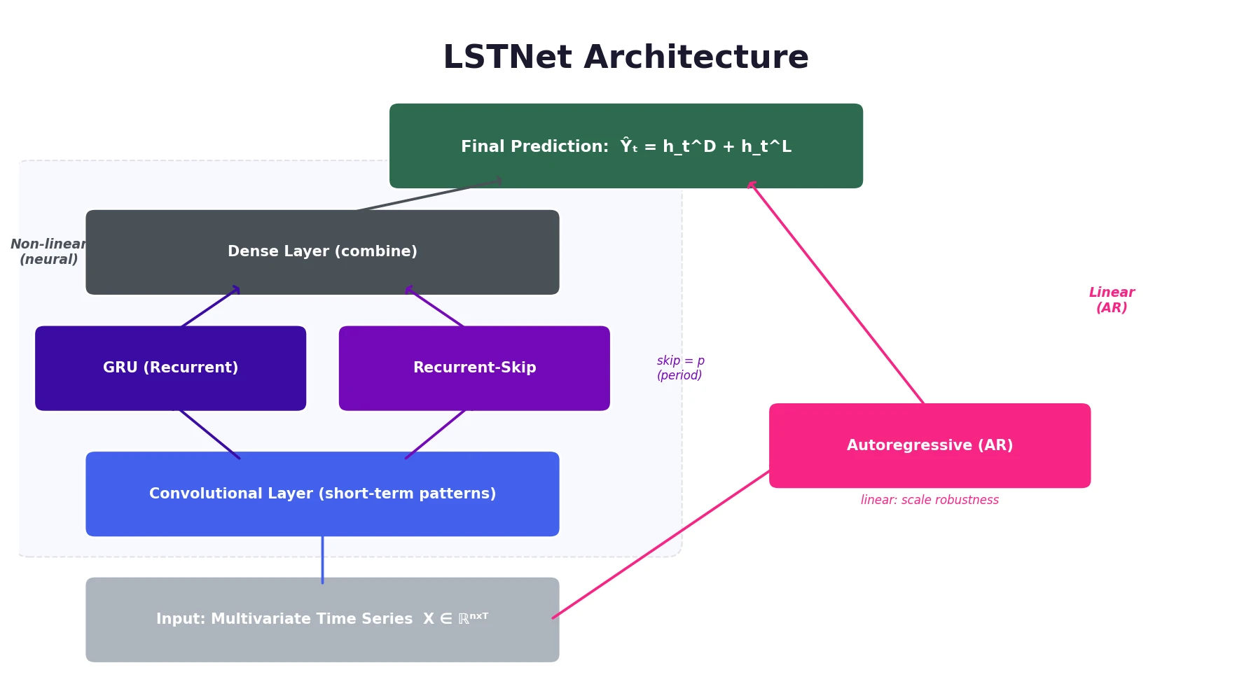
This is a Method paper that introduces the Long- and Short-term Time-series Network (LSTNet), a deep learning architecture specifically designed for multivariate time series forecasting. LSTNet combines convolutional neural networks (CNNs), recurrent neural networks (RNNs) with a novel skip-connection structure, and a traditional autoregressive (AR) component into a unified framework. The architecture targets the challenge of simultaneously capturing both short-term local dependencies and long-term periodic patterns in temporal data.
Why Short-Term and Long-Term Patterns Need Separate Treatment
Real-world multivariate time series often exhibit a mixture of repeating patterns at different time scales. Highway traffic, for example, shows daily peaks (morning vs. evening commutes) alongside weekly patterns (weekday vs. weekend behavior). Solar energy output varies with cloud movements on short time scales and with seasonal daylight changes on longer ones. Electricity consumption follows similar daily and weekly cycles.
Traditional autoregressive methods (VAR, ARIMA) and Gaussian Process models struggle to distinguish and jointly model these two kinds of recurring patterns. Standard RNNs, including LSTM and GRU variants, theoretically handle long-range dependencies but in practice suffer from gradient vanishing when the period length is large (e.g., 24 hours at hourly resolution, or 168 time steps for weekly patterns). The authors also identify a scale sensitivity problem: neural network models can fail when the magnitude of the input signal changes in non-periodic ways, such as sudden shifts in electricity consumption due to holidays or weather events.
Combining CNNs, Recurrent-Skip Connections, and Autoregression
The LSTNet architecture consists of four main components that work together.
Convolutional Component
The first layer applies 1D convolution without pooling across the multivariate input. Each filter has width $\omega$ (in the time dimension) and height $n$ (spanning all variables), producing feature maps that capture short-term local dependency patterns among variables:
$$h_k = \text{RELU}(W_k * X + b_k)$$
where $*$ denotes convolution and the input is zero-padded so each output vector has length $T$. The output is a $d_c \times T$ matrix where $d_c$ is the number of filters.
Recurrent Component
The CNN output feeds into a GRU-based recurrent layer that uses RELU (rather than the standard tanh) as the hidden update activation:
$$\begin{aligned} r_t &= \sigma(x_t W_{xr} + h_{t-1} W_{hr} + b_r) \\ u_t &= \sigma(x_t W_{xu} + h_{t-1} W_{hu} + b_u) \\ c_t &= \text{RELU}(x_t W_{xc} + r_t \odot (h_{t-1} W_{hc}) + b_c) \\ h_t &= (1 - u_t) \odot h_{t-1} + u_t \odot c_t \end{aligned}$$
Recurrent-Skip Component
The key architectural innovation is a recurrent structure with temporal skip connections. Instead of connecting to the immediately preceding hidden state $h_{t-1}$, skip links connect to the hidden state from $p$ steps ago ($h_{t-p}$), where $p$ corresponds to the period length of the data (e.g., $p = 24$ for hourly data with daily periodicity):
$$\begin{aligned} r_t &= \sigma(x_t W_{xr} + h_{t-p} W_{hr} + b_r) \\ u_t &= \sigma(x_t W_{xu} + h_{t-p} W_{hu} + b_u) \\ c_t &= \text{RELU}(x_t W_{xc} + r_t \odot (h_{t-p} W_{hc}) + b_c) \\ h_t &= (1 - u_t) \odot h_{t-p} + u_t \odot c_t \end{aligned}$$
This design shortens the effective path length for learning periodic dependencies, making optimization easier. A dense layer combines outputs from both recurrent components:
$$h_t^D = W^R h_t^R + \sum_{i=0}^{p-1} W_i^S h_{t-i}^S + b$$
Temporal Attention Alternative
For datasets without clear periodicity, LSTNet offers an attention-based variant (LSTNet-Attn) as an alternative to the recurrent-skip component. The attention mechanism learns to weight hidden representations across the input window adaptively. The attention weights $\alpha_t \in \mathbb{R}^q$ at time $t$ are computed as:
$$\alpha_t = \text{AttnScore}(H_t^R, h_{t-1}^R)$$
where $H_t^R = [h_{t-q}^R, \dots, h_{t-1}^R]$ stacks the RNN hidden representations column-wise and AttnScore is a similarity function (dot product, cosine, or a parameterized MLP). The weighted context vector and final output are:
$$\begin{aligned} c_t &= H_t \alpha_t \\ h_t^D &= W[c_t;; h_{t-1}^R] + b \end{aligned}$$
Autoregressive Component
To address the scale insensitivity of neural networks, LSTNet adds a classical autoregressive model in parallel:
$$h_{t,i}^L = \sum_{k=0}^{q^{ar}-1} W_k^{ar} y_{t-k,i} + b^{ar}$$
The final prediction integrates both the neural network and AR outputs:
$$\hat{Y}_t = h_t^D + h_t^L$$
This decomposition separates the prediction into a linear part (handling local scale changes) and a non-linear part (capturing recurring patterns).
Objective Function
LSTNet supports two loss functions, selected via validation performance. The default is the squared (L2) loss:
$$\underset{\Theta}{\text{minimize}} \sum_{t \in \Omega_{\text{Train}}} \left| Y_t - \hat{Y}_{t-h} \right|_F^2$$
Motivated by the strong performance of Linear SVR baselines, LSTNet also supports the absolute (L1) loss, which is more robust to anomalies in real time series data:
$$\underset{\Theta}{\text{minimize}} \sum_{t \in \Omega_{\text{Train}}} \sum_{i=0}^{n-1} \left| Y_{t,i} - \hat{Y}_{t-h,i} \right|$$
where $\Theta$ is the full parameter set, $\Omega_{\text{Train}}$ is the set of training time stamps, $|\cdot|_F$ is the Frobenius norm, and $h$ is the forecast horizon.
Evaluation on Four Benchmark Datasets
Datasets
| Dataset | Length | Variables | Sample Rate |
|---|---|---|---|
| Traffic | 17,544 | 862 | 1 hour |
| Solar-Energy | 52,560 | 137 | 10 minutes |
| Electricity | 26,304 | 321 | 1 hour |
| Exchange-Rate | 7,588 | 8 | 1 day |
All datasets are split 60/20/20 (train/validation/test) in chronological order. Traffic, Solar-Energy, and Electricity exhibit clear periodic patterns (daily and weekly), while Exchange-Rate shows only short-term local continuity.
Baselines
The authors compare against seven methods: AR (univariate autoregression), LRidge (VAR with L2 regularization), LSVR (VAR with SVR objective), TRMF (temporal regularized matrix factorization), GP (Gaussian Process), VAR-MLP (hybrid MLP-autoregressive), and RNN-GRU (standard GRU).
Metrics
Two evaluation metrics are used:
- Root Relative Squared Error (RSE) (lower is better): A scaled RMSE that normalizes by the standard deviation of the test data, making comparison across datasets readable regardless of data scale:
$$\text{RSE} = \frac{\sqrt{\sum_{(i,t) \in \Omega_{\text{Test}}} (Y_{it} - \hat{Y}_{it})^2}}{\sqrt{\sum_{(i,t) \in \Omega_{\text{Test}}} (Y_{it} - \text{mean}(Y))^2}}$$
- Empirical Correlation Coefficient (CORR) (higher is better): The average Pearson correlation between predicted and true time series across all $n$ variables:
$$\text{CORR} = \frac{1}{n} \sum_{i=1}^{n} \frac{\sum_t (Y_{it} - \text{mean}(Y_i))(\hat{Y}_{it} - \text{mean}(\hat{Y}_i))}{\sqrt{\sum_t (Y_{it} - \text{mean}(Y_i))^2 \sum_t (\hat{Y}_{it} - \text{mean}(\hat{Y}_i))^2}}$$
Main Results
The models are evaluated at horizons $h \in {3, 6, 12, 24}$, corresponding to 3-24 hours for Traffic and Electricity, 30-240 minutes for Solar-Energy, and 3-24 days for Exchange-Rate.
LSTNet-Skip achieved the best result in 17 out of 32 (dataset, metric, horizon) combinations, and LSTNet-Attn won 7 more. No other method won more than 3. At horizon 24, the best LSTNet variant improved over RNN-GRU by 9.2% RSE on Solar-Energy (LSTNet-Attn), 11.7% on Traffic (LSTNet-Skip), and 22.2% on Electricity (LSTNet-Skip). On the Exchange-Rate dataset, which lacks periodic patterns, LSTNet performed comparably to AR and LRidge, as expected.
Ablation Study
Removing each component individually revealed:
- Without AR: The largest performance drops across most datasets, confirming the AR component’s role in handling scale changes. Visualization showed that LSTNet-Skip successfully tracks sudden magnitude shifts in electricity consumption around the 1000th hour, while the model without AR fails.
- Without Skip/CNN: Significant drops on datasets with periodic patterns, though less consistent than removing AR.
- Full LSTNet: The most robust configuration across all datasets and horizons.
A simulation experiment with synthetic autoregressive data confirmed that standard RNN-GRU fails to track non-periodic scale changes, while LSTNet with its AR component adapts properly.
Robust Performance Through Architectural Complementarity
LSTNet’s main strength is the complementarity of its components. The CNN captures short-term local patterns, the recurrent-skip layer captures long-term periodic dependencies, and the AR component provides robustness to scale changes. On datasets with strong periodicity (Traffic, Solar-Energy, Electricity), the skip connections provide large gains. On datasets without periodicity (Exchange-Rate), the AR component prevents degradation below competitive baselines.
The primary limitation is that the skip length $p$ in the recurrent-skip component must be manually specified or tuned. For datasets with known periodicity (e.g., hourly data with daily cycles), $p$ is straightforward to set. For datasets without clear periodicity, $p$ must be tuned as a hyperparameter, and the attention-based variant (LSTNet-Attn) offers an alternative that avoids this requirement. Future work directions include automatic period detection and incorporating variable-level attribute information into the convolutional layer.
Reproducibility Details
Data
| Purpose | Dataset | Size | Notes |
|---|---|---|---|
| Training/Evaluation | Traffic | 17,544 x 862 | California DoT highway occupancy, hourly, 2015-2016 |
| Training/Evaluation | Solar-Energy | 52,560 x 137 | Solar power from 137 PV plants in Alabama, 10-min intervals, 2006 |
| Training/Evaluation | Electricity | 26,304 x 321 | kWh consumption for 321 clients, hourly, 2012-2014 |
| Training/Evaluation | Exchange-Rate | 7,588 x 8 | Daily exchange rates for 8 countries, 1990-2016 |
All datasets are publicly available via the GitHub repository.
Algorithms
- Optimizer: Adam
- Dropout: 0.1 or 0.2 after each layer except input and output
- Window size $q$: grid search over ${2^0, 2^1, \ldots, 2^9}$
- Skip length $p$: set to 24 for Traffic/Electricity; tuned from $2^1$ to $2^6$ for Solar-Energy/Exchange-Rate
- Objective: L2 loss (Eq. 7) or L1 loss (Eq. 9), selected via validation
Models
- Hidden dimensions (Recurrent/CNN): ${50, 100, 200}$
- Hidden dimensions (Recurrent-skip): ${20, 50, 100}$
- AR regularization: ${0.1, 1, 10}$
Evaluation
| Metric | Best LSTNet RSE | Baseline (RNN-GRU) | Improvement |
|---|---|---|---|
| Solar-Energy (h=24) | 0.4403 (Attn) | 0.4852 | 9.2% |
| Traffic (h=24) | 0.4973 (Skip) | 0.5633 | 11.7% |
| Electricity (h=24) | 0.1007 (Skip) | 0.1295 | 22.2% |
Hardware
Not specified in the paper.
Artifacts
| Artifact | Type | License | Notes |
|---|---|---|---|
| LSTNet (laiguokun/LSTNet) | Code | MIT | Official PyTorch implementation (Python 2.7, PyTorch 0.3.0) |
| Multivariate Time Series Data (laiguokun/multivariate-time-series-data) | Dataset | Unknown | Preprocessed benchmark datasets (Traffic, Solar-Energy, Electricity, Exchange-Rate) |
Reproducibility status: Highly Reproducible. Code and all four benchmark datasets are publicly available. Hyperparameter search ranges are fully specified.
Paper Information
Citation: Lai, G., Chang, W.-C., Yang, Y., & Liu, H. (2018). Modeling Long- and Short-Term Temporal Patterns with Deep Neural Networks. The 41st International ACM SIGIR Conference on Research & Development in Information Retrieval (SIGIR ‘18), 95-104. https://doi.org/10.1145/3209978.3210006
@inproceedings{lai2018modeling,
  title={Modeling Long- and Short-Term Temporal Patterns with Deep Neural Networks},
  author={Lai, Guokun and Chang, Wei-Cheng and Yang, Yiming and Liu, Hanxiao},
  booktitle={The 41st International ACM SIGIR Conference on Research \& Development in Information Retrieval},
  pages={95--104},
  year={2018},
  doi={10.1145/3209978.3210006}
}