A Method for Learning Arbitrary Lagrangians
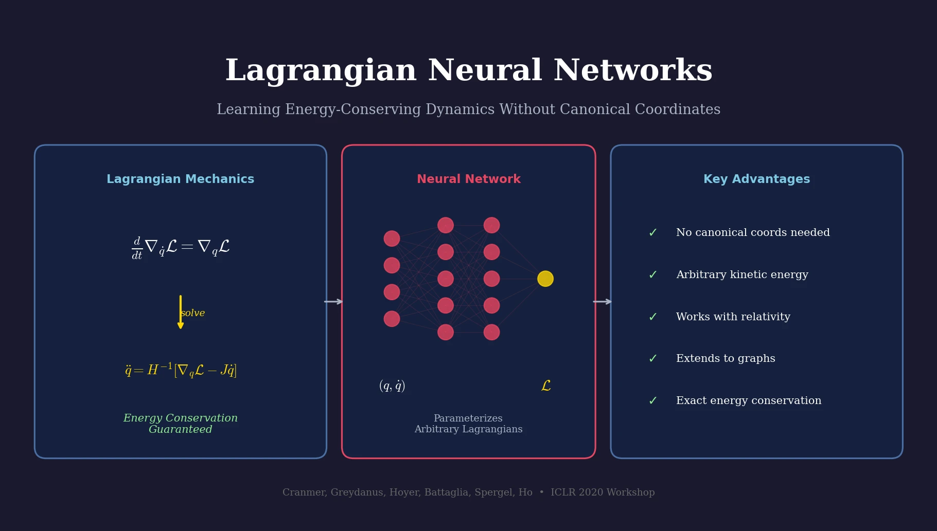
This is a Method paper that introduces Lagrangian Neural Networks (LNNs), a neural network architecture that parameterizes arbitrary Lagrangians to learn energy-conserving dynamics from data. The key contribution is showing that neural networks can learn Lagrangian functions directly, and that the Euler-Lagrange equation can be solved numerically using automatic differentiation to produce physically consistent dynamics. The approach is strictly more general than prior methods: it does not require canonical coordinates (unlike Hamiltonian Neural Networks) and does not restrict the functional form of kinetic energy (unlike Deep Lagrangian Networks).
Why Standard Neural Networks Fail at Conservation Laws
Neural networks struggle to learn fundamental symmetries and conservation laws from data. A standard neural network trained on trajectories of a double pendulum will gradually dissipate energy over long rollouts, producing physically implausible behavior. This happens because unconstrained function approximators have no inductive bias toward conservation.
Hamiltonian Neural Networks (HNNs) addressed this by learning a Hamiltonian function, which automatically enforces energy conservation. However, the Hamiltonian formalism requires inputs in canonical coordinates $(q, p)$ satisfying strict Poisson bracket relations:
$$ p_i \equiv \frac{\partial \mathcal{L}}{\partial \dot{q}_i} \quad \Longleftrightarrow \quad {q_i, q_j} = 0, \quad {p_i, p_j} = 0, \quad {q_i, p_j} = \delta_{ij} $$
In many real-world settings, the canonical momenta are unknown or difficult to compute. For example, in special relativity the canonical momentum $\dot{q}(1 - \dot{q}^2)^{-3/2}$ is a complex nonlinear function of velocity. Deep Lagrangian Networks (DeLaNs) partially addressed this by learning Lagrangians, but they assumed kinetic energy takes the rigid-body form $T = \dot{q}^T M \dot{q}$, which excludes relativistic and other non-standard systems.
Solving Euler-Lagrange for a Black-Box Lagrangian
The core innovation of LNNs is a method for computing accelerations from a neural network that represents an arbitrary Lagrangian $\mathcal{L}(q, \dot{q})$. Starting from the Euler-Lagrange equation:
$$ \frac{d}{dt} \nabla_{\dot{q}} \mathcal{L} = \nabla_{q} \mathcal{L} $$
The authors expand the time derivative using the chain rule, yielding:
$$ \left(\nabla_{\dot{q}} \nabla_{\dot{q}}^{\top} \mathcal{L}\right) \ddot{q} + \left(\nabla_{q} \nabla_{\dot{q}}^{\top} \mathcal{L}\right) \dot{q} = \nabla_{q} \mathcal{L} $$
Solving for the accelerations gives:
$$ \ddot{q} = \left(\nabla_{\dot{q}} \nabla_{\dot{q}}^{\top} \mathcal{L}\right)^{-1} \left[ \nabla_{q} \mathcal{L} - \left(\nabla_{q} \nabla_{\dot{q}}^{\top} \mathcal{L}\right) \dot{q} \right] $$
This requires computing the Hessian of the neural network with respect to $\dot{q}$ and then inverting it (using a pseudoinverse for numerical stability). JAX’s automatic differentiation makes this feasible in just a few lines of code, despite the seemingly complex chain of second-order derivatives. The matrix inverse scales as $\mathcal{O}(d^3)$ with the number of coordinates $d$.
A critical implementation detail is the choice of activation function. Since the method takes second-order derivatives of the network, ReLU is unsuitable (its second derivative is zero everywhere). After a hyperparameter search over ReLU$^2$, ReLU$^3$, tanh, sigmoid, and softplus, the authors found softplus performed best.
The authors also developed a custom initialization scheme, using symbolic regression to find initialization variances that maintain well-conditioned gradients through the Hessian computation:
$$ \sigma = \frac{1}{\sqrt{n}} \begin{cases} 2.2 & \text{First layer} \\ 0.58i & \text{Hidden layer } i \\ n & \text{Output layer} \end{cases} $$
Extension to Graphs and Continuous Systems
LNNs extend naturally to graph-structured and continuous systems via Lagrangian Graph Networks. For a system with $n$ gridpoints, the total Lagrangian is decomposed into local densities:
$$ \mathcal{L} = \sum_{i=1}^{n} \mathcal{L}_i, \quad \text{where} \quad \mathcal{L}_i = \mathcal{L}_{\text{density}}\left({\phi_j, \dot{\phi}_j}_{j \in \mathcal{I}_i}\right) $$
Here $\mathcal{I}_i$ defines the neighborhood of node $i$ (e.g., ${i-1, i, i+1}$ for a 1D grid). The Lagrangian density is modeled as an MLP. The resulting Hessian matrix is sparse, with non-zero entries only at “neighbor of neighbor” positions, enabling efficient computation: in 1D, only 5 forward-over-backward autodiff passes are needed, and the tridiagonal inverse runs in linear time.
Experiments: Double Pendulum, Relativity, and Waves
All models used 4-layer MLPs with 500 hidden units, softplus activations, a decaying learning rate starting at $10^{-3}$, and batch size 32.
Double Pendulum
The LNN and baseline achieved similar instantaneous acceleration losses ($7.3$ vs. $7.4 \times 10^{-2}$). The key difference appeared in long-term energy conservation: averaged over 40 random initial conditions with 100 time steps, the mean energy discrepancy was 8% of max potential energy for the baseline but only 0.4% for the LNN.
Relativistic Particle
For a particle with Lagrangian $\mathcal{L} = ((1 - \dot{q}^2)^{-1/2} - 1) + gq$, the canonical momenta $\dot{q}(1 - \dot{q}^2)^{-3/2}$ are non-trivial. An HNN trained on non-canonical coordinates $(q, \dot{q})$ failed to learn the dynamics. The LNN succeeded using the same non-canonical coordinates, matching the performance of an HNN given the correct canonical coordinates.
1D Wave Equation
The Lagrangian Graph Network learned the wave equation dynamics ($\ddot{\phi} = \frac{\partial^2 \phi}{\partial x^2}$ with $c = 1$) on a 100-gridpoint domain with periodic boundary conditions. The network learned the Lagrangian density corresponding to the continuum form $\mathcal{L} = \int (\dot{\phi}^2 - (\partial \phi / \partial x)^2) dx$, accurately modeling wave propagation and conserving energy across the material.
| Experiment | Model | Energy Error (% of max PE) | Canonical Coords Required |
|---|---|---|---|
| Double Pendulum | Baseline | 8% | N/A |
| Double Pendulum | LNN | 0.4% | No |
| Relativistic Particle | HNN (non-canonical) | Failed | Yes |
| Relativistic Particle | HNN (canonical) | Succeeded | Yes |
| Relativistic Particle | LNN | Succeeded | No |
| 1D Wave Equation | LGN | Energy conserved | No |
Findings and Comparison to Prior Approaches
LNNs combine several desirable properties that no single prior method offers:
| Property | Neural Net | Neural ODE | HNN | DeLaN | LNN |
|---|---|---|---|---|---|
| Models dynamical systems | Yes | Yes | Yes | Yes | Yes |
| Learns differential equations | Yes | Yes | Yes | Yes | |
| Learns exact conservation laws | Yes | Yes | Yes | ||
| Learns from arbitrary coordinates | Yes | Yes | Yes | Yes | |
| Learns arbitrary Lagrangians | Yes |
The main limitation is computational cost: the Hessian computation and inversion scale as $\mathcal{O}(d^3)$ in the number of coordinates. The Lagrangian Graph Network partially mitigates this for spatially extended systems through the sparsity of the resulting Hessian. The method also assumes access to state derivatives ($\dot{q}$) during training, which may not always be directly available from observations.
Reproducibility Details
Data
| Purpose | Dataset | Size | Notes |
|---|---|---|---|
| Training | Double pendulum | 600,000 random initial conditions | Simulated with masses and lengths set to 1 |
| Training | Relativistic particle | Random initial conditions and $g$ values | $c = 1$, mass = 1, uniform potential |
| Training | 1D wave equation | 100 gridpoints | Periodic boundary conditions, $c = 1$ |
Algorithms
- Forward model: Euler-Lagrange equation solved via Equation 6 using JAX autodiff
- Pseudoinverse used for Hessian inversion to handle potential singular matrices
- Custom initialization scheme (Equation 16) derived via symbolic regression with eureqa
- Softplus activation selected via hyperparameter search
Models
- 4-layer MLP with 500 hidden units for all experiments
- Softplus activation function
- Code: github.com/MilesCranmer/lagrangian_nns (Apache-2.0)
Evaluation
| Metric | LNN | Baseline | Notes |
|---|---|---|---|
| Acceleration loss (double pendulum) | $7.3 \times 10^{-2}$ | $7.4 \times 10^{-2}$ | Similar short-term accuracy |
| Energy error (double pendulum) | 0.4% | 8% | Percentage of max potential energy |
Hardware
Not specified in the paper. JAX-based implementation supports CPU and GPU execution.
Reproducibility Status: Highly Reproducible
Artifacts
| Artifact | Type | License | Notes |
|---|---|---|---|
| lagrangian_nns | Code | Apache-2.0 | Official JAX implementation with notebooks for all experiments |
| Training data | Dataset | N/A | Generated procedurally; simulation code included in repository |
| Trained models | Model | N/A | Not provided |
Paper Information
Citation: Cranmer, M., Greydanus, S., Hoyer, S., Battaglia, P., Spergel, D., & Ho, S. (2020). Lagrangian Neural Networks. ICLR 2020 Workshop on Integration of Deep Neural Models and Differential Equations. arXiv: 2003.04630
Publication: ICLR 2020 Workshop on Integration of Deep Neural Models and Differential Equations
@misc{cranmer2020lagrangian,
  title={Lagrangian Neural Networks},
  author={Cranmer, Miles and Greydanus, Sam and Hoyer, Stephan and Battaglia, Peter and Spergel, David and Ho, Shirley},
  year={2020},
  eprint={2003.04630},
  archiveprefix={arXiv},
  primaryclass={cs.LG}
}