A General-Purpose Edge Convolution Module for Point Cloud Learning
This is a Method paper that introduces EdgeConv, a neural network module for learning on point clouds. The key idea is to construct a local graph structure and define convolution-like operations over edges connecting neighboring points. Unlike prior graph neural network approaches that operate on a fixed graph, DGCNN (Dynamic Graph CNN) recomputes the graph at each layer using k-nearest neighbors in feature space. This dynamic graph update allows the network to learn semantic groupings that differ from spatial proximity, enabling information propagation across long distances in the original point cloud. The model achieves strong results on classification (ModelNet40), part segmentation (ShapeNetPart), and semantic segmentation (S3DIS) benchmarks.
Why Point Clouds Need Topology Recovery
Point clouds are the raw output of most 3D acquisition devices (LiDAR, stereo reconstruction) and serve as the simplest geometric representation for countless applications in graphics, robotics, and autonomous driving. However, point clouds inherently lack topological information: they are unordered sets of points with no connectivity structure.
Standard CNNs require grid-structured input, making them incompatible with irregular point cloud data. Volumetric approaches that discretize point clouds onto 3D grids introduce quantization artifacts and excessive memory usage. PointNet addressed this by operating on each point independently and aggregating with a symmetric function (max pooling), achieving permutation invariance. However, this independence means PointNet cannot capture local geometric structure.
PointNet++ partially addresses this by applying PointNet hierarchically in local neighborhoods, but it constructs neighborhoods based on Euclidean distances in the input space and does not update the graph structure during processing. The fundamental limitation is that treating points independently, even locally, prevents the model from learning the geometric relationships between points that carry important structural and semantic information.
EdgeConv: Combining Local Geometry with Global Structure
Given an $F$-dimensional point cloud $\mathbf{X} = \lbrace \mathbf{x}_1, \ldots, \mathbf{x}_n \rbrace \subseteq \mathbb{R}^F$, DGCNN constructs a directed graph $\mathcal{G} = (\mathcal{V}, \mathcal{E})$ as the $k$-nearest neighbor graph in $\mathbb{R}^F$, including self-loops so each node also points to itself. Edge features are defined as:
$$ \mathbf{x}_i’ = \square_{j:(i,j) \in \mathcal{E}} h_\Theta(\mathbf{x}_i, \mathbf{x}_j) $$
where $h_\Theta$ is a learnable nonlinear function and $\square$ denotes a channel-wise symmetric aggregation operation (e.g., max or sum).
The choice of edge function $h_\Theta$ determines the model’s properties. The authors analyze several options:
| Choice | Edge function | Properties |
|---|---|---|
| Standard convolution | $\theta_m \cdot \mathbf{x}_j$ | Requires fixed grid structure |
| PointNet | $h_\Theta(\mathbf{x}_i)$ | Global only, ignores local structure |
| PointNet++ | $h_\Theta(\mathbf{x}_j)$ | Local only, loses global context |
| Local difference | $h_\Theta(\mathbf{x}_j - \mathbf{x}_i)$ | Local patches without global positioning |
| EdgeConv (this work) | $\bar{h}_\Theta(\mathbf{x}_i, \mathbf{x}_j - \mathbf{x}_i)$ | Both local geometry and global structure |
The concrete EdgeConv operation uses an asymmetric edge function that combines the point’s own features $\mathbf{x}_i$ (global shape structure) with the relative difference $\mathbf{x}_j - \mathbf{x}_i$ (local neighborhood information):
$$ e’_{ijm} = \text{ReLU}(\boldsymbol{\theta}_m \cdot (\mathbf{x}_j - \mathbf{x}_i) + \boldsymbol{\phi}_m \cdot \mathbf{x}_i) $$
$$ x’_{im} = \max_{j:(i,j) \in \mathcal{E}} e’_{ijm} $$
where $\boldsymbol{\Theta} = (\theta_1, \ldots, \theta_M, \phi_1, \ldots, \phi_M)$ are learnable parameters. This formulation can be implemented as a shared MLP followed by max pooling over neighbors.
Dynamic Graph Recomputation
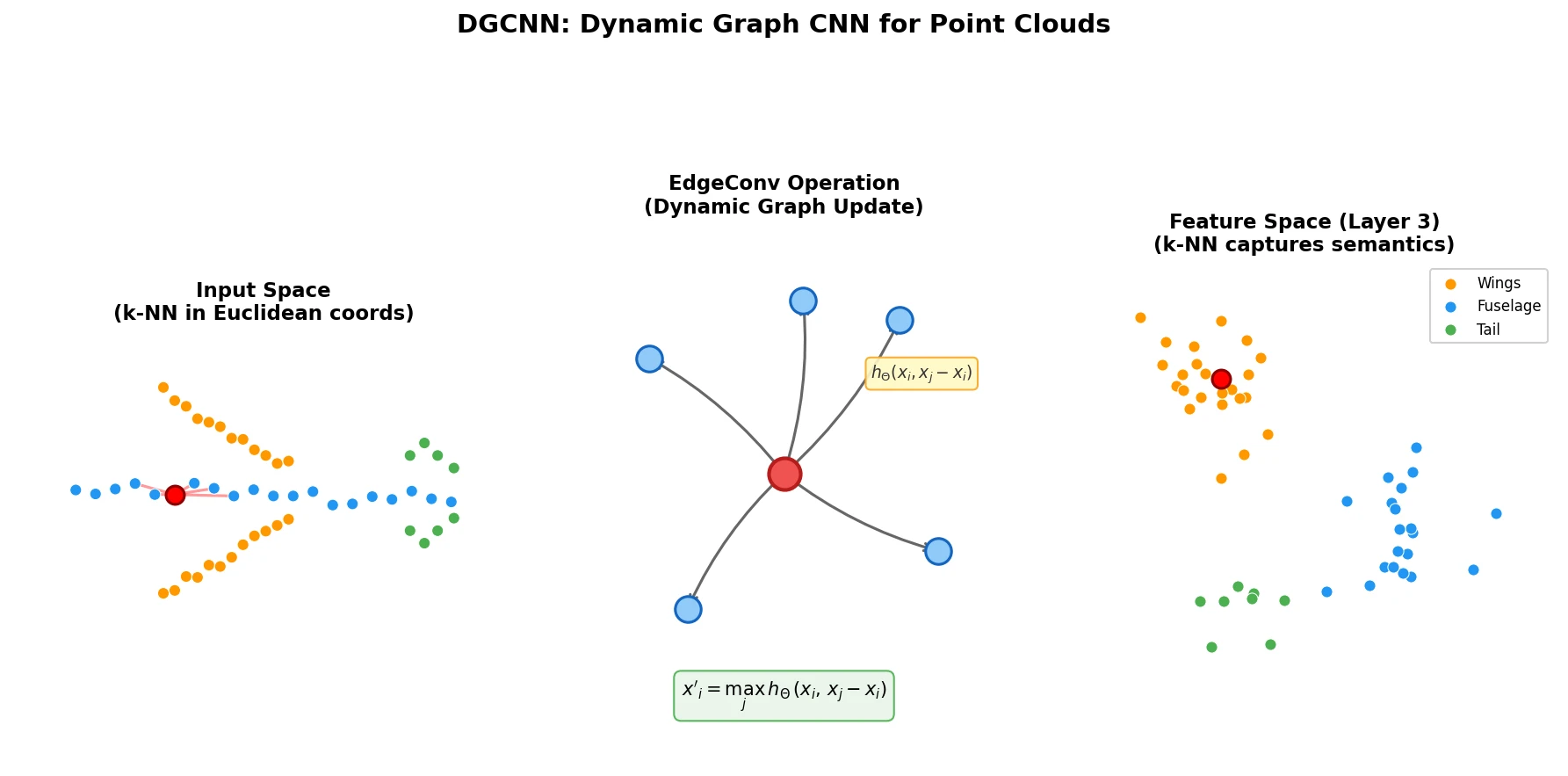
The defining feature of DGCNN is that the graph $\mathcal{G}^{(l)}$ is recomputed at each layer $l$ using k-NN in the current feature space, rather than being fixed based on input coordinates. This means:
- The receptive field grows to be as large as the diameter of the point cloud while remaining sparse.
- Points that are far apart in Euclidean space but semantically similar (e.g., the two wings of an airplane) become neighbors in deeper feature spaces.
- The model learns to construct the graph itself, rather than taking it as a fixed input.
Permutation and Translation Invariance
EdgeConv is permutation invariant because the max aggregation is a symmetric function. It has a “partial” translation invariance property: the local difference term $\mathbf{x}_j - \mathbf{x}_i$ is fully translation invariant, while the global term $\boldsymbol{\phi}_m \cdot \mathbf{x}_i$ is translation-dependent. Setting $\boldsymbol{\phi}_m = 0$ yields full translation invariance but loses global positioning information.
Benchmarks: Classification, Part Segmentation, and Scene Segmentation
Classification on ModelNet40
The classification architecture uses four EdgeConv layers with output dimensions (64, 64, 128, 256), $k = 20$ nearest neighbors, and shortcut connections that concatenate all EdgeConv outputs into a $64 + 64 + 128 + 256 = 512$-dimensional per-point feature. A shared fully-connected layer (1024) aggregates these multi-scale features. Global max and sum pooling produce a 1D descriptor, followed by two fully-connected layers (512, 256) with dropout (probability 0.5). All layers use LeakyReLU and batch normalization. Input point clouds are rescaled to fit into the unit sphere.
Training uses SGD with momentum 0.9, initial learning rate 0.1, cosine annealing to 0.001, and batch size 32. Batch normalization momentum is 0.9 with no BN decay. Data augmentation includes random scaling and perturbation of object and point locations. The value of $k$ is selected using an 80/20 train/validation split, then the model is retrained on the full training set.
| Method | Mean Class Acc. (%) | Overall Acc. (%) |
|---|---|---|
| PointNet | 86.0 | 89.2 |
| PointNet++ | – | 90.7 |
| PointCNN | 88.1 | 92.2 |
| PCNN | – | 92.3 |
| DGCNN (baseline, fixed graph) | 88.9 | 91.7 |
| DGCNN | 90.2 | 92.9 |
| DGCNN (2048 points) | 90.7 | 93.5 |
Model Complexity
DGCNN achieves a favorable tradeoff between model size, inference speed, and accuracy:
| Method | Model Size (MB) | Time (ms) | Accuracy (%) |
|---|---|---|---|
| PointNet (baseline) | 9.4 | 6.8 | 87.1 |
| PointNet | 40 | 16.6 | 89.2 |
| PointNet++ | 12 | 163.2 | 90.7 |
| PCNN | 94 | 117.0 | 92.3 |
| DGCNN (baseline) | 11 | 19.7 | 91.7 |
| DGCNN | 21 | 27.2 | 92.9 |
The DGCNN baseline outperforms PointNet++ by 1.0% while being 7x faster. The full DGCNN outperforms PCNN by 0.6% while being 4x faster with 4.5x fewer parameters.
Ablation Studies
| Centralization | Dynamic Graph | 2048 Points | Mean Class (%) | Overall (%) |
|---|---|---|---|---|
| 88.9 | 91.7 | |||
| x | 89.3 | 92.2 | ||
| x | x | 90.2 | 92.9 | |
| x | x | x | 90.7 | 93.5 |
The choice of $k$ also matters:
| $k$ | Mean Class Acc. (%) | Overall Acc. (%) |
|---|---|---|
| 5 | 88.0 | 90.5 |
| 10 | 88.9 | 91.4 |
| 20 | 90.2 | 92.9 |
| 40 | 89.4 | 92.4 |
$k = 20$ performs best on 1024 points. Larger $k$ (e.g., 40) degrades performance because Euclidean distance poorly approximates geodesic distance at larger scales for a given point density.
Part Segmentation on ShapeNetPart
On the ShapeNetPart dataset (16,881 shapes, 16 categories, 50 part labels), DGCNN achieves 85.2% mean IoU, comparable to PointNet++ (85.1%) and PointCNN (86.1%). The model also demonstrates robustness to partial data, maintaining reasonable segmentation quality even when half of the points are removed.
Indoor Scene Segmentation on S3DIS
On the Stanford Large-Scale 3D Indoor Spaces Dataset (6 indoor areas, 272 rooms, 13 semantic categories), DGCNN achieves 56.1% mean IoU and 84.1% overall accuracy using 6-fold cross-validation over the areas, outperforming PointNet (47.6% / 78.5%) and producing smoother segmentation boundaries. Each point is represented as a 9D vector (XYZ, RGB, and normalized spatial coordinates), with 4,096 points sampled per $1\text{m} \times 1\text{m}$ block during training.
Semantic Feature Spaces and Future Directions
A key qualitative finding is that the feature spaces learned by DGCNN in deeper layers capture semantic similarity rather than spatial proximity. Visualizations show that semantically similar structures (e.g., all legs of a table, or all wings of an airplane) are brought close together in feature space, even when they are far apart in the original 3D embedding. This property also transfers across shapes: features from one airplane’s wing are close to the wing features of a different airplane in the learned feature space.
The authors identify several directions for future work:
- Efficiency: Incorporating fast data structures (e.g., KD-trees) instead of computing pairwise distances for k-NN queries.
- Higher-order relationships: Considering tuples of points rather than only pairwise relationships.
- Non-shared transformations: Applying different transformations to different local patches rather than using shared weights.
- Abstract point clouds: Extending the approach to non-geometric applications like document retrieval and image processing, where the role of geometry in abstract feature spaces may provide new insights.
The model has some limitations. On S3DIS, PointCNN achieves notably higher mean IoU (65.39% vs. 56.1%), suggesting room for improvement on large-scale scene segmentation. The dynamic k-NN computation adds overhead relative to fixed-graph approaches, though the overall model remains efficient.
Reproducibility Details
Data
| Purpose | Dataset | Size | Notes |
|---|---|---|---|
| Classification | ModelNet40 | 12,311 CAD models (40 categories) | 1,024 points uniformly sampled per model |
| Part Segmentation | ShapeNetPart | 16,881 shapes (16 categories, 50 parts) | 2,048 points per shape |
| Scene Segmentation | S3DIS | 272 rooms (13 categories) | 4,096 points per 1m x 1m block |
Algorithms
- k-NN graph construction: Pairwise distance matrix in feature space, $k = 20$ (classification) or $k = 40$ (2048 points).
- EdgeConv: Shared MLP on concatenated $[\mathbf{x}_i, \mathbf{x}_j - \mathbf{x}_i]$ features, followed by channel-wise max pooling over neighbors.
- Dynamic graph update: Graph recomputed from k-NN in feature space at each EdgeConv layer.
Models
- Classification: 4 EdgeConv layers (64, 64, 128, 256) + shortcut concatenation (512-dim) + shared FC (1024) + global max/sum pooling + FC (512, 256). 21 MB.
- Segmentation: Spatial transformer + 3 EdgeConv layers + shared FC (1024) aggregation + shortcut connections + FC (256, 256, 128).
- All layers use LeakyReLU and batch normalization. Dropout 0.5 in final FC layers.
Evaluation
| Task | Metric | DGCNN | Best Baseline |
|---|---|---|---|
| ModelNet40 Classification | Overall Accuracy | 92.9% | 92.3% (PCNN) |
| ShapeNetPart Segmentation | Mean IoU | 85.2% | 86.1% (PointCNN) |
| S3DIS Scene Segmentation | Mean IoU | 56.1% | 65.39% (PointCNN) |
Artifacts
| Artifact | Type | License | Notes |
|---|---|---|---|
| WangYueFt/dgcnn | Code | MIT | Official TensorFlow and PyTorch implementations |
Hardware
- Training used NVIDIA TITAN X GPUs. Distributed training (2 GPUs) for part segmentation.
- Forward pass time: 27.2 ms per sample (1,024 points) on a single GPU.
Paper Information
Citation: Wang, Y., Sun, Y., Liu, Z., Sarma, S. E., Bronstein, M. M., & Solomon, J. M. (2019). Dynamic Graph CNN for Learning on Point Clouds. ACM Transactions on Graphics, 38(5), Article 146. https://doi.org/10.1145/3326362
Code: github.com/WangYueFt/dgcnn (MIT License)
@article{wang2019dynamic,
  title={Dynamic Graph CNN for Learning on Point Clouds},
  author={Wang, Yue and Sun, Yongbin and Liu, Ziwei and Sarma, Sanjay E. and Bronstein, Michael M. and Solomon, Justin M.},
  journal={ACM Transactions on Graphics},
  volume={38},
  number={5},
  articleno={146},
  pages={1--12},
  year={2019},
  publisher={ACM},
  doi={10.1145/3326362}
}