What kind of paper is this?
This is primarily a Method paper, with significant Theory contributions.
The authors propose a specific algorithm (“InterFlow”) for constructing generative models based on continuous-time normalizing flows. The work is characterized by the derivation of a new training objective (a simple quadratic loss) that bypasses the computational bottlenecks of previous methods. It includes prominent baseline comparisons against continuous flow methods (FFJORD, OT-Flow) and diffusion models. The theoretical component establishes the validity of the interpolant density satisfying the continuity equation (a conservation law governing how probability mass flows) and bounds the Wasserstein-2 distance (a measure of transport cost between distributions, penalizing squared displacement) of the transport.
What is the motivation?
The primary motivation is to overcome the computational inefficiency of training Continuous Normalizing Flows (CNFs) using Maximum Likelihood Estimation (MLE). Standard CNF training requires backpropagating through numerical ODE solvers, which is costly and limits scalability.
Additionally, while score-based diffusion models (SDEs) have achieved high sample quality, they theoretically require infinite time integration and rely on specific noise schedules. The authors aim to establish a method that works strictly with Probability Flow ODEs on finite time intervals, retaining the flexibility to connect arbitrary densities without the complexity of SDEs or the cost of standard ODE adjoint methods.
What is the novelty here?
The core novelty is the Stochastic Interpolant framework:
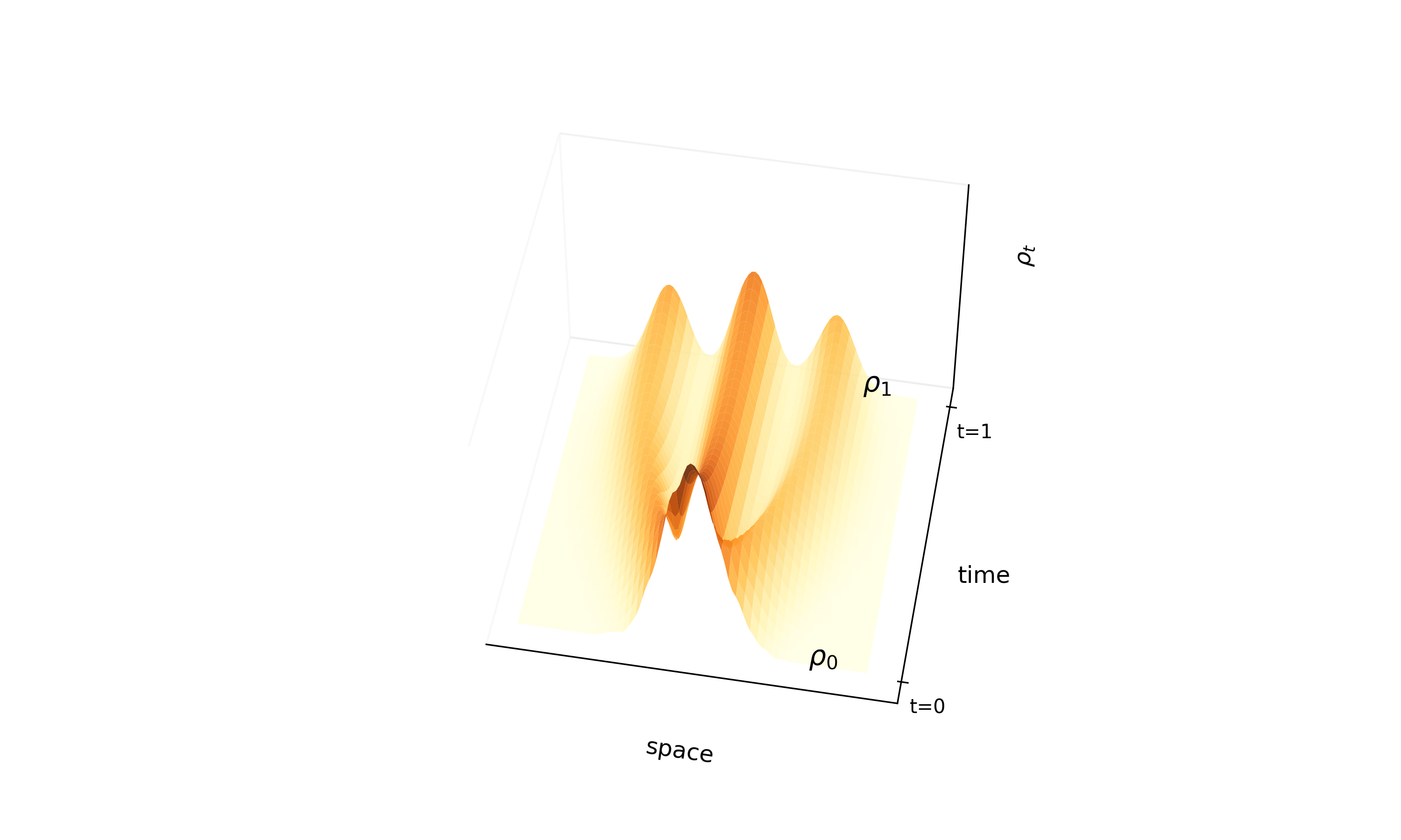
- Explicit Interpolant Construction: The method defines a time-dependent interpolant $x_t = I_t(x_0, x_1)$ (e.g., trigonometric interpolation) that connects samples from the base density $\rho_0$ and target $\rho_1$.
- Simulation-Free Training: The velocity field $v_t(x)$ of the probability flow is learned by minimizing a simple quadratic objective: $G(\hat{v}) = \mathbb{E}[|\hat{v}_t(x_t)|^2 - 2\partial_t x_t \cdot \hat{v}_t(x_t)]$. Because $\partial_t I_t$ is known analytically from the interpolant definition, the expectation can be estimated by sampling $(x_0, x_1, t)$ directly. This avoids ODE integration during training (ODE integration is still required at inference).
- Decoupling Path and Optimization: The choice of path (interpolant) is separated from the optimization of the velocity field. MLE methods couple the path and objective.
- Connection to Score-Based Models: The authors show that for Gaussian base densities and trigonometric interpolants, the learned velocity field is explicitly related to the score function $\nabla \log \rho_t$, providing a theoretical bridge between CNFs and diffusion models.
What experiments were performed?
The authors performed validation across synthetic, tabular, and image domains:
- 2D Density Estimation: Benchmarked on “Checkerboard”, “8 Gaussians”, and anisotropic curved densities to visualize mode coverage and transport smoothness.
- High-Dimensional Tabular Data: Evaluated on standard benchmarks (POWER, GAS, HEPMASS, MINIBOONE, BSDS300) comparing Negative Log Likelihood (NLL) against FFJORD, OT-Flow, and others.
- Image Generation: Trained models on CIFAR-10 ($32 \times 32$), ImageNet ($32 \times 32$), and Oxford Flowers ($128 \times 128$) to test scalability.
- Ablations: Investigated optimizing the interpolant path itself (e.g., learning Fourier coefficients for the path) to approach optimal transport and minimize path length.
What outcomes/conclusions?
- Performance: The method matches or supersedes conventional ODE flows (like FFJORD) in terms of NLL while being significantly cheaper to train.
- Efficiency: The training cost per epoch is constant (simulation-free), whereas MLE-based ODE methods see growing costs as the dynamics become more complex.
- Scalability: The method successfully scales to $128 \times 128$ resolution on a single GPU, a resolution that prior ab-initio ODE flows had not demonstrated.
- Flexibility: The framework can connect any two arbitrary densities (e.g., connecting two different complex 2D distributions) without needing one to be Gaussian.
- Optimal Transport: For a fixed interpolant, minimizing $G(\hat{v})$ over the velocity field recovers the velocity for that specific path. Additionally optimizing over the interpolant family yields a solution to the Benamou-Brenier optimal transport problem.
- Limitations: The authors acknowledge that image FID scores trail dedicated diffusion models, noting that InterFlow was not optimized with standard training tricks such as exponential moving averages, truncation, or learning rate warm-ups. The framework’s sample quality could likely improve with these additions.
Reproducibility Details
Data
- Tabular Datasets: POWER (6D), GAS (8D), HEPMASS (21D), MINIBOONE (43D), BSDS300 (63D).
- Training points range from ~30k (MINIBOONE) to ~1.6M (POWER).
- Image Datasets:
- CIFAR-10 ($32 \times 32$, 50k training points).
- ImageNet ($32 \times 32$, ~1.28M training points).
- Oxford Flowers ($128 \times 128$, ~315k training points).
- Time Sampling: Time $t$ is sampled from a Beta distribution during training (reweighting) to focus learning near the target.
Algorithms
- Interpolant: The primary interpolant used is trigonometric: $I_t(x_0, x_1) = \cos(\frac{\pi t}{2})x_0 + \sin(\frac{\pi t}{2})x_1$.
- Alternative linear interpolant: $I_t = a_t x_0 + b_t x_1$.
- Loss Function:
$$G(\hat{v}) = \mathbb{E}_{t, x_0, x_1}[|\hat{v}_t(x_t)|^2 - 2\partial_t I_t(x_0, x_1) \cdot \hat{v}_t(x_t)]$$
- The expectation is amenable to empirical estimation using batches of $x_0, x_1, t$.
- Sampling: Numerical integration using Dormand-Prince (Runge-Kutta 4/5).
- Optimization: SGD/Adam variants used for optimization.
Models
- Tabular Architectures:
- Feed-forward networks with 4-5 hidden layers.
- Hidden widths: 512 (POWER, GAS, HEPMASS, MINIBOONE) or 1024 (BSDS300).
- Activation: ReLU (general) or ELU (BSDS300).
- Image Architectures:
- U-Net based on the DDPM implementation.
- Dimensions: 256 hidden dimension.
- Sinusoidal time embeddings used.
Evaluation
- Metrics: Negative Log Likelihood (NLL) in nats (tabular) or bits per dim (images), Frechet Inception Distance (FID) for images.
- Baselines: FFJORD, Glow, Real NVP, OT-Flow, ScoreFlow, DDPM.
Tabular NLL (nats, lower is better; Table 2 Left):
| Method | POWER | GAS | HEPMASS | MINIBOONE | BSDS300 |
|---|---|---|---|---|---|
| MADE | 3.08 | -3.56 | 20.98 | 15.59 | -148.85 |
| Real NVP | -0.17 | -8.33 | 18.71 | 13.55 | -153.28 |
| Glow | -0.17 | -8.15 | 18.92 | 11.35 | -155.07 |
| CPF | -0.52 | -10.36 | 16.93 | 10.58 | -154.99 |
| NSP | -0.64 | -13.09 | 14.75 | 9.67 | -157.54 |
| FFJORD | -0.46 | -8.59 | 14.92 | 10.43 | -157.40 |
| OT-Flow | -0.30 | -9.20 | 17.32 | 10.55 | -154.20 |
| Ours | -0.57 | -12.35 | 14.85 | 10.42 | -156.22 |
Image Generation NLL and FID (Table 2 Right; NLL in bits per dim, lower is better):
| Method | CIFAR-10 NLL | CIFAR-10 FID | ImageNet-32 NLL | ImageNet-32 FID |
|---|---|---|---|---|
| FFJORD | 3.40 | - | - | - |
| Glow | 3.35 | - | 4.09 | - |
| DDPM | ≤3.75 | 3.17 | - | - |
| DDPM++ (Song et al., 2021) | ≤3.37 | 2.90 | - | - |
| ScoreSDE (Song et al., 2021) | 2.99 | 2.92 | - | - |
| VDM | ≤2.65 | 7.41 | ≤3.72 | - |
| Soft Truncation | 2.88 | 3.45 | 3.85 | 8.42 |
| ScoreFlow | 2.81 | 5.40 | 3.76 | 10.18 |
| Ours | 2.99 | 10.27 | 3.48 | 8.49 |
Note: DDPM++ is from Song et al. (2021), the same work as ScoreSDE (it is the architecture optimized for VP/sub-VP SDEs). InterFlow matches ScoreSDE on CIFAR-10 NLL (2.99 bits per dim) while being simulation-free. FID is weaker than dedicated image models (10.27 vs 2.92 for ScoreSDE), reflecting the paper’s primary focus on tractable likelihood rather than sample quality.
Hardware
- Compute: All models were trained on a single NVIDIA A100 GPU.
- Training Time:
- Tabular: $10^5$ steps.
- Images: $1.5 \times 10^5$ to $6 \times 10^5$ steps.
- Speedup: Demonstrated ~400x speedup compared to FFJORD on MiniBooNE dataset.
Artifacts
| Artifact | Type | License | Notes |
|---|---|---|---|
| lucidrains/denoising-diffusion-pytorch (link defunct) | Code | MIT | Base U-Net architecture used for image experiments; original GitHub account no longer available |
No official code release accompanies this paper. All tabular datasets (POWER, GAS, HEPMASS, MINIBOONE, BSDS300) are publicly available from prior work. CIFAR-10 and ImageNet are standard public benchmarks. Oxford Flowers 102 is also publicly available. Hyperparameters and architectures are fully specified in Tables 3 and 4 of the paper.
Paper Information
Citation: Albergo, M. S., & Vanden-Eijnden, E. (2023). Building Normalizing Flows with Stochastic Interpolants. The Eleventh International Conference on Learning Representations.
Publication: ICLR 2023
@inproceedings{albergoBuildingNormalizingFlows2022,
  title = {Building {{Normalizing Flows}} with {{Stochastic Interpolants}}},
  booktitle = {The {{Eleventh International Conference}} on {{Learning Representations}}},
  author = {Albergo, Michael Samuel and {Vanden-Eijnden}, Eric},
  year = 2023,
  url = {https://openreview.net/forum?id=li7qeBbCR1t}
}
Additional Resources: