Neural ODEs: Continuous-Depth Deep Learning

Key Prerequisites: Before diving in, note that for the ODE solver to guarantee a unique solution, the neural network $f(h(t), t, \theta)$ parameterizing the dynamics must be Lipschitz continuous. This ensures the Picard-Lindelöf theorem holds, preventing trajectories from crossing and guaranteeing a well-defined backward pass.

What kind of paper is this?

This is primarily a Method paper, with a strong secondary Theory component.

• Method: It proposes a novel family of deep neural network models where the derivative of the hidden state is parameterized by a neural network. It provides specific algorithms (Algorithm 1) for training these models scalably.
• Theory: It derives the adjoint sensitivity method for backpropagating through black-box ODE solvers and proves the “Instantaneous Change of Variables” theorem (Theorem 1) for continuous normalizing flows.

What is the motivation?

The authors aim to address limitations in discrete deep learning architectures:

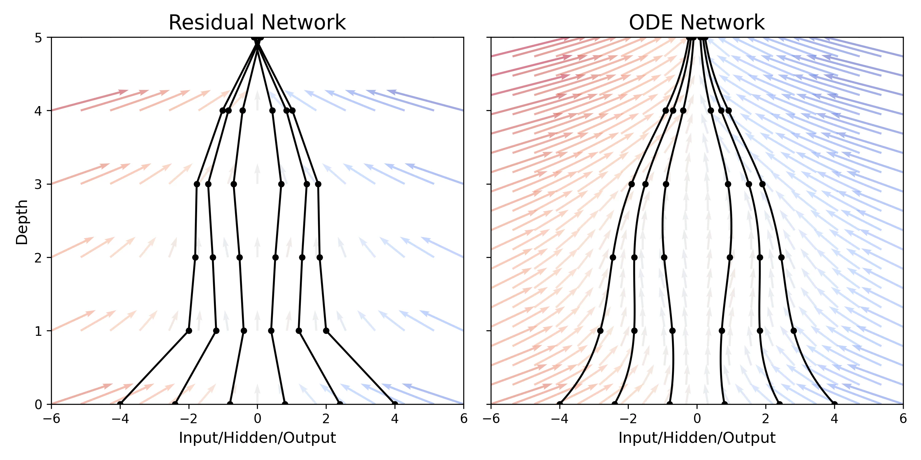
• Discrete vs. Continuous: Existing models like Residual Networks build transformations by composing discrete steps, which can be seen as an Euler discretization of a continuous transformation. The authors investigate the limit as step sizes go to zero.
• Memory Efficiency: Backpropagating through deep discrete networks requires storing intermediate activations, leading to linear memory cost in terms of depth, which is a major bottleneck.
• Irregular Data: Recurrent Neural Networks (RNNs) struggle with data arriving at arbitrary times, typically requiring discretization into fixed bins.
• Normalizing Flow Costs: Standard normalizing flows have a bottleneck in computing the determinant of the Jacobian, which is computationally expensive ($O(D^3)$).

What is the novelty here?

The core contribution is the Neural ODE formulation: $$\frac{dh(t)}{dt} = f(h(t), t, \theta)$$ where the output is computed using a black-box differential equation solver.

Key technical innovations include:

1. Adjoint Sensitivity Method for Backprop: The authors treat the solver as a black box and compute gradients by solving a second, augmented ODE backwards in time. This allows for constant memory cost regardless of depth.
2. Adaptive Computation: The model uses modern ODE solvers that adapt evaluation steps based on error tolerance, allowing the model to trade precision for speed explicitly.
3. Continuous Normalizing Flows (CNF): By moving to continuous time, the change of variables formula simplifies from a log-determinant (cubic cost) to a trace operation (linear cost), enabling scalable generative modeling.
4. Latent ODEs: A generative time-series model that represents time-series as latent trajectories determined by a local initial state and global shared dynamics, handling irregular sampling naturally.

What experiments were performed?

The authors validated the method across three distinct domains:

1. Supervised Learning (MNIST):
   • Compared ODE-Net against a standard ResNet and a Runge-Kutta network (RK-Net).
   • Measured test error, parameter count, and memory usage.
   • Analyzed the trade-off between numerical precision (tolerance) and speed (NFE).
2. Continuous Normalizing Flows (Generative):
   • Compared CNF against standard Normalizing Flows (NF) on density estimation tasks using toy 2D datasets (Target, Two Circles, Two Moons).
   • Evaluated training loss (KL divergence) and maximum likelihood estimation.
3. Time-Series Modeling (Latent ODE):
   • Tested on a dataset of bi-directional spirals with irregular timestamps and Gaussian noise.
   • Compared Latent ODEs against RNNs and RNNs with time-concatenation on predictive RMSE.

What were the outcomes and conclusions drawn?

• Efficiency: ODE-Nets achieved roughly equivalent accuracy to ResNets on MNIST (0.42% vs 0.41% error) but with constant memory cost ($O(1)$) compared to ResNet’s linear cost ($O(L)$).
• Adaptive Depth: The number of function evaluations (NFE) in ODE-Nets increases with training epoch, suggesting the model adapts its complexity as it learns.
• Generative Performance: Continuous Normalizing Flows (CNF) achieved lower loss than standard NFs and were easier to train, as they can expand capacity via width ($M$).
• Irregular Time-Series: Latent ODEs significantly outperformed RNNs on irregular spiral data (0.1346 RMSE vs 0.1813 RMSE), learning interpretable latent trajectories that could switch direction smoothly.

Critical Analysis

Despite their elegance, Neural ODEs introduce significant theoretical and practical challenges:

1. Growing NFE (Computational Cost): As training progresses, the learned dynamics often become “stiff,” requiring the adaptive solver to take increasingly smaller steps to maintain error tolerance. This can make inference prohibitively slow compared to fixed-depth ResNets.
2. Numerical Instability: Integrating backward in time (for the adjoint method) is numerically unstable for many systems. Trajectories that converge forward will diverge backward, potentially leading to inaccurate gradients.
3. Topological Constraints: Because ODE trajectories cannot cross (due to uniqueness), Neural ODEs cannot model functions that require intersecting trajectories (e.g., the “gdonut” problem) without lifting the state into higher dimensions (Augmented Neural ODEs).

Reproducibility Details

Data

• MNIST: Standard handwritten digit dataset used for supervised learning benchmarks.
• Toy 2D Densities: “Two Circles” and “Two Moons” distributions used for visualizing normalizing flows.
• Bi-directional Spirals: A generated dataset of 1,000 2D spirals (half clockwise, half counter-clockwise). Sampled at 100 irregular timesteps with added Gaussian noise. Subsampled to $n={30, 50, 100}$ points for training.

Algorithms

1. Adjoint Sensitivity Method (Backpropagation)

To optimize the parameters of the ODE-Net, the authors use the adjoint sensitivity method to compute gradients. Standard backpropagation would require storing the activations at every step of the ODE solver, incurring a high memory cost that scales linearly with the number of steps.

Instead, this method treats the ODE solver as a “black box” and computes gradients by solving a second, augmented ODE backwards in time from the final state $t_1$ to the initial state $t_0$.

The augmented state contains three components that are solved simultaneously:

1. The State: The original hidden state $z(t)$, which is reconstructed backwards.
2. The Adjoint: The sensitivity of the loss with respect to the state, $a(t) = \partial L / \partial z(t)$.
3. The Gradient: The accumulating gradients with respect to parameters, $\partial L / \partial \theta$.

The dynamics of this augmented system are defined as: $$\frac{d}{dt}\begin{bmatrix} z(t) \ a(t) \ \partial L/\partial \theta \end{bmatrix} = \begin{bmatrix} f(z(t), t, \theta) \ -a(t)^T \frac{\partial f}{\partial z} \ -a(t)^T \frac{\partial f}{\partial \theta} \end{bmatrix}$$

Using this approach, the vector-Jacobian products (e.g., $a(t)^T \frac{\partial f}{\partial z}$) are evaluated efficiently using automatic differentiation.

Why: Reconstructing $z(t)$ backwards avoids storing the forward pass, enabling constant memory cost ($O(1)$) regardless of depth.

Origin: Adapted from Pontryagin’s maximum principle (1962) for optimal control.

import torch
import torch.nn as nn
from torchdiffeq import odeint_adjoint

class ODEFunc(nn.Module):
    def __init__(self, dim):
        super(ODEFunc, self).__init__()
        self.net = nn.Sequential(
            nn.Linear(dim, 50),
            nn.Tanh(),
            nn.Linear(50, dim),
        )

    def forward(self, t, y):
        # Defines dy/dt = f(y, t)
        return self.net(y)

# Usage with adjoint method for O(1) memory backprop
func = ODEFunc(dim=2)
y0 = torch.tensor([[1., 0.]]) # Initial state
t = torch.linspace(0., 1., 10) # Time points to solve for

# 'odeint_adjoint' automatically handles the augmented state backward pass
out = odeint_adjoint(func, y0, t, method='dopri5')

2. Instantaneous Change of Variables (CNF)

For generative modeling, the authors introduce Continuous Normalizing Flows (CNF). In discrete normalizing flows, the probability density of a transformed variable is calculated using the change of variables theorem, which requires computing the log-determinant of the Jacobian: $\log p(z_1) = \log p(z_0) - \log |\det \frac{\partial z_1}{\partial z_0}|$. This operation is computationally expensive ($O(D^3)$) and often restricts model architectures to ensure the Jacobian is easy to compute (e.g., triangular).

Moving to continuous time simplifies this requirement. The paper proves that if the transformation is defined by an ODE, the change in log-probability follows a differential equation determined by the trace of the Jacobian: $$\frac{\partial \log p(z(t))}{\partial t} = -\text{tr}\left( \frac{\partial f}{\partial z(t)} \right)$$

The total change in log-density is obtained by integrating this value over time.

def get_trace(y, f):
    """
    Computes trace of Jacobian df/dy.
    For high dimensions, use Hutchinson's trace estimator (approximate).
    """
    tr = 0.
    for i in range(y.size(1)):
        # Gradients of f's i-th component w.r.t y's i-th component
        tr += torch.autograd.grad(f[:, i].sum(), y, create_graph=True)[0][:, i]
    return tr

# In the ODE function:
# d(log_p)/dt = -trace(df/dy)

Why: The trace operator has linear cost ($O(D)$), whereas the determinant has cubic cost ($O(D^3)$). This allows for unrestricted, “wide” architectures that are automatically bijective.

Origin: This is the “Instantaneous Change of Variables” theorem (Theorem 1), derived in Appendix A of the paper.

Models

ODE-Net (MNIST Classification):

• Input: Downsamples input twice.
• Core: 6 standard residual blocks replaced by a single ODESolve module.
• Output: Global average pooling + Fully connected layer.
• Solver: Implicit Adams method.

class ODEBlock(nn.Module):
    def __init__(self, odefunc):
        super(ODEBlock, self).__init__()
        self.odefunc = odefunc
        self.integration_time = torch.tensor([0, 1]).float()

    def forward(self, x):
        self.integration_time = self.integration_time.type_as(x)
        # Returns [x(t0), x(t1)]; we only want final state x(t1)
        out = odeint_adjoint(self.odefunc, x, self.integration_time)
        return out[1]

# ResNet-like architecture with ODE block
model = nn.Sequential(
    nn.Conv2d(1, 64, 3, 1),
    nn.ReLU(inplace=True),
    ODEBlock(ODEFunc(64)), # Continuous-depth layer replacement
    nn.BatchNorm2d(64),
    nn.AdaptiveAvgPool2d((1, 1)),
    nn.Flatten(),
    nn.Linear(64, 10)
)

Latent ODE (Time-Series):

• Encoder: RNN with 25 hidden units processing data backwards to produce $q(z_0|x)$. It runs backwards so the final RNN state summarizes the entire sequence at $t_0$, parameterizing the initial latent state $z_0$ for the forward-running ODE.
• Latent Space: 4-dimensional latent state $z_0$.
• Dynamics ($f$): Neural network with one hidden layer of 20 units.
• Decoder: Neural network with one hidden layer of 20 units computing $p(x_{t_i}|z_{t_i})$.
• Likelihood: Poisson process likelihood $\lambda(z(t))$ used for modeling event rates.

Evaluation

Hardware

• Implementation: Hidden state dynamics evaluated on GPU using TensorFlow.
• Solvers: Fortran ODE solvers (LSODE, VODE) from scipy.integrate were used for the actual integration.
• Note: While the original paper used TensorFlow/Scipy, the authors later released torchdiffeq (PyTorch), which has become the standard implementation for this architecture. The code samples above reflect this modern standard.
• Interface: Python’s autograd framework bridged the TensorFlow dynamics and Scipy solvers.

Citation & Resources

Citation: Chen, R. T. Q., Rubanova, Y., Bettencourt, J., & Duvenaud, D. (2018). Neural ordinary differential equations. Proceedings of the 32nd International Conference on Neural Information Processing Systems, 6572–6583.

Publication: NeurIPS 2018

Additional Resources:

• Official PyTorch Implementation

@inproceedings{chen2018neural,
  title={Neural ordinary differential equations},
  author={Chen, Ricky T. Q. and Rubanova, Yulia and Bettencourt, Jesse and Duvenaud, David},
  booktitle={Proceedings of the 32nd International Conference on Neural Information Processing Systems},
  pages={6572--6583},
  year={2018}
}