What kind of paper is this?
This is a Method paper.
It identifies a specific failure mode in existing neural network methodologies (least-squares regression on multi-valued inverse problems) and proposes a novel architecture (combining MLPs with Mixture Models) to solve it. It derives the mathematical framework for training this architecture via standard back-propagation and validates it against the established baseline.
What is the motivation?
Standard neural networks trained with sum-of-squares (MSE) or cross-entropy error functions approximate the conditional average of the target data, $\langle t|x \rangle$.
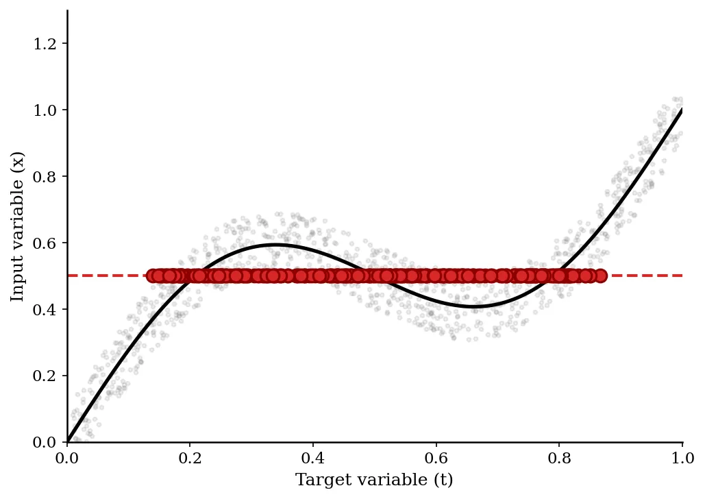
While optimal for single-valued functions or classification, this produces completely erroneous results for inverse problems where the mapping is multi-valued (one input has multiple valid outputs). For example, in robot inverse kinematics, “elbow-up” and “elbow-down” configurations can achieve the same hand position. An MSE-trained network will average these two valid angles, resulting in an invalid configuration (the paper shows this produces end-effector positions at the outer boundary of the accessible region, corresponding to $\theta_2 = \pi$).

What is the novelty here?
The introduction of the Mixture Density Network (MDN).
The neural network predicts the parameters (mixing coefficients, means, and variances) of a kernel mixture distribution (typically Gaussian).

Key technical contributions include:
- Architecture: Mapping network outputs to mixture parameters using specific activation functions to satisfy constraints (Softmax for priors $\alpha$, Exponential for variances $\sigma$).
- Training: Deriving the error function as the negative log-likelihood of the mixture model.
- Optimization: Deriving the exact derivatives (gradients) of the error with respect to network outputs, allowing the mixture model parameters to be learned via standard back-propagation.
What experiments were performed?
Bishop validated the method on two tasks, comparing an MDN against a standard MLP trained with least-squares:
- Toy Inverse Problem: A sinusoidal mapping $x = t + 0.3\sin(2\pi t) + \epsilon$. The forward problem ($t \to x$) is single-valued, but the inverse ($x \to t$) is multi-valued.
- Robot Kinematics: A 2-link robot arm simulation. The task is to map end-effector Cartesian coordinates $(x_1, x_2)$ back to joint angles $(\theta_1, \theta_2)$.
What outcomes/conclusions?
- Toy Problem: The standard least-squares network failed completely, drawing a smooth curve through the average of the multiple branches, which did not correspond to valid data. The MDN correctly modeled the tri-modal density and discontinuous jumps in the most probable solution.
- Robot Kinematics: The MDN reduced the RMS positioning error by an order of magnitude compared to the standard network (0.0053 vs 0.0578).
- Generality: The paper concludes that MDNs provide a complete description of the conditional probability density, allowing users to calculate any statistic (mean, mode, variance) needed for the application.
Extracting Predictions
Once trained, the MDN outputs a full conditional density $p(t|x)$, from which several useful statistics can be derived:
- Conditional mean: $\langle t|x \rangle = \sum_i \alpha_i(x) \mu_i(x)$, equivalent to the standard least-squares network output.
- Conditional variance: $s^2(x) = \sum_i \alpha_i(x) { \sigma_i(x)^2 + | \mu_i(x) - \sum_j \alpha_j(x) \mu_j(x) |^2 }$, which is input-dependent (more general than the constant-variance least-squares assumption).
- Most probable branch: Select the kernel $i$ with the largest mixing coefficient $\alpha_i(x)$, then use its center $\mu_i$ as the prediction. This yields a discontinuous but accurate mapping for multi-valued problems.
Limitations
- Model order selection: The number of mixture components $m$ must be chosen in advance. The paper acknowledges this as an open problem and suggests cross-validation or Bayesian model comparison as potential approaches.
- Computational overhead: The number of network outputs grows as $(c + 2) \times m$, where $c$ is the target dimensionality. For high-dimensional targets or many kernels, this can become significant.
- Isotropic kernels: The paper uses a single variance parameter $\sigma_i$ per kernel (shared across target dimensions), which assumes isotropic covariance. The paper notes this can be generalized to full covariance matrices at the cost of additional parameters.
Reproducibility Details
Data
1. Toy Inverse Problem
- Function: $x = t + 0.3\sin(2\pi t) + \epsilon$
- Noise: $\epsilon \sim U(-0.1, 0.1)$
- Sampling: 1,000 points generated by sampling $t$ at equal intervals in range $(0, 1)$.
- Task: Inverse mapping (predict $t$ given $x$).
2. Robot Kinematics
- System: 2-link arm with lengths $L_1=0.8, L_2=0.2$.
- Forward Kinematics:
- $x_1 = L_1 \cos(\theta_1) - L_2 \cos(\theta_1 + \theta_2)$
- $x_2 = L_1 \sin(\theta_1) - L_2 \sin(\theta_1 + \theta_2)$
- Constraints: $\theta_1 \in (0.3, 1.2)$, $\theta_2 \in (\pi/2, 3\pi/2)$.
- Dataset: 1,000 training points, 1,000 test points.
Algorithms
Mixture Model Definition
The conditional density is defined as:
$$p(t|x) = \sum_{i=1}^{m} \alpha_i(x) \phi_i(t|x)$$
Where kernels $\phi_i$ are Gaussians with centers $\mu_i(x)$ and variances $\sigma_i(x)$.
Network Output Mappings
If the network produces raw outputs $z$, they are mapped to parameters as follows to satisfy probability constraints:
- Mixing Coefficients ($\alpha$): Softmax. $\alpha_i = \frac{\exp(z_i^\alpha)}{\sum_j \exp(z_j^\alpha)}$
- Variances ($\sigma$): Exponential. $\sigma_i = \exp(z_i^\sigma)$
- Means ($\mu$): Linear/Identity. $\mu_{ik} = z_{ik}^\mu$
Loss Function
Negative Log Likelihood:
$$E^q = - \ln \left{ \sum_{i=1}^{m} \alpha_i(x^q) \phi_i(t^q|x^q) \right}$$
Models
1. Toy Problem Configuration
- Structure: MLP with 1 input ($x$), 1 hidden layer.
- Hidden Units: 20 units (tanh activation).
- Outputs: 9 units.
- $m=3$ Gaussian kernels.
- Parameters per kernel: 1 $\alpha$, 1 $\sigma$, 1 $\mu$. Total = $3 \times 3 = 9$.
- Training: 1,000 cycles of BFGS.
2. Robot Kinematics Configuration (Least-Squares Baseline)
- Structure: MLP with 2 inputs ($x_1, x_2$), 2 linear outputs ($\theta_1, \theta_2$).
- Hidden Units: Best result with 20 units (tanh activation), tested with 5, 10, 15, 20, 25, 30.
- Training: 3,000 cycles of BFGS.
3. Robot Kinematics Configuration (MDN)
- Structure: MLP with 2 inputs ($x_1, x_2$).
- Hidden Units: 10 units (tanh activation).
- Outputs: 8 units.
- $m=2$ Gaussian kernels.
- Target dimension $c=2$ (predicting $\theta_1, \theta_2$).
- Parameters per kernel: 1 $\alpha$ + 1 $\sigma$ (common variance) + 2 $\mu$ (means for $\theta_1, \theta_2$).
- Total = $2 \times (1 + 1 + 2) = 8$.
Evaluation
Metric: RMS Euclidean distance between the desired end-effector position and the achieved position (calculated by plugging predicted angles back into forward kinematics).
| Model | Hidden Units | Kernels | RMS Error |
|---|---|---|---|
| Least Squares | 20 | N/A | 0.0578 |
| MDN | 10 | 2 | 0.0053 |
Paper Information
Citation: Bishop, C. M. (1994). Mixture Density Networks. Neural Computing Research Group Report: NCRG/94/004, Aston University.
Publication: Neural Computing Research Group Technical Report 1994
@techreport{bishopMixtureDensityNetworks1994,
  title = {Mixture {{Density Networks}}},
  author = {Bishop, Christopher M.},
  year = 1994,
  month = feb,
  number = {NCRG/94/004},
  institution = {Aston University}
}