What kind of paper is this?
This is a Method paper that introduces the Importance Weighted Autoencoder (IWAE), a generative model that shares the same architecture as the Variational Autoencoder (VAE) but uses a different, tighter objective function. The key innovation is using importance weighting to derive a strictly tighter log-likelihood lower bound than the standard VAE objective.
What is the motivation?
The standard VAE has several limitations that motivated this work:
- Strong assumptions: VAEs typically assume the posterior distribution is simple (e.g., approximately factorial) and that its parameters can be easily approximated from observations.
- Simplified representations: The VAE objective can force models to learn overly simplified representations that underutilize the network’s full modeling capacity.
- Harsh penalization: The VAE objective harshly penalizes approximate posterior samples that are poor explanations for the data, which can be overly restrictive.
- Inactive units: VAEs tend to learn latent spaces with effective dimensions far below their capacity, where many latent units are ignored (a phenomenon later termed posterior collapse, where the approximate posterior collapses to the prior and conveys no information). The authors wanted to investigate whether a new objective could address this issue.
What is the novelty here?
The core novelty is the IWAE objective function, denoted as $\mathcal{L}_{k}$.
VAE ($\mathcal{L}_{1}$ Bound): The standard VAE maximizes $\mathcal{L}(x)=\mathbb{E}_{q(h|x)}[\log\frac{p(x,h)}{q(h|x)}]$. This is equivalent to the new bound when $k=1$.
IWAE ($\mathcal{L}_{k}$ Bound): The IWAE maximizes a tighter bound that uses $k$ samples drawn from the recognition model $q(h|x)$:
$$\mathcal{L}_{k}(x)=\mathbb{E}_{h_{1},…,h_{k}\sim q(h|x)}\left[\log\frac{1}{k}\sum_{i=1}^{k}\frac{p(x,h_{i})}{q(h_{i}|x)}\right]$$
Tighter Bound: The authors prove that this bound is always tighter than or equal to the VAE bound ($\mathcal{L}_{k+1} \geq \mathcal{L}_{k}$) and that as $k$ approaches infinity, $\mathcal{L}_{k}$ approaches the true log-likelihood $\log p(x)$.
Increased Flexibility: Using multiple samples gives the IWAE additional flexibility to learn generative models whose posterior distributions are complex and violate the VAE’s simplifying assumptions.
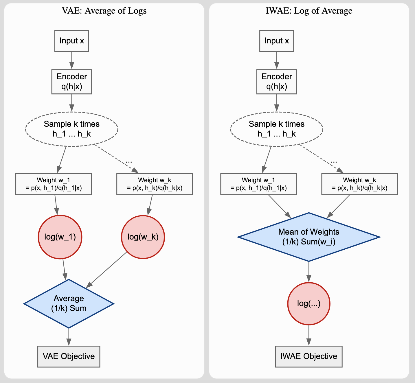
Key Concept: Averaging Inside vs. Outside the Log
A crucial distinction exists between how VAE and IWAE utilize $k$ samples. Understanding this difference explains why increasing $k$ in IWAE improves the bound. In VAE, it reduces variance.
. IWAE averages the weights first then takes the log (log of average)")
VAE (Average of Logs):
For a VAE, using $k$ samples approximates:
$$\mathbb{E}\left[ \frac{1}{k} \sum_{i=1}^k \log w_i \right] \approx \text{ELBO}$$
where $w_i = p(x, h_i) / q(h_i | x)$. Increasing $k$ here only reduces the variance of the gradient estimator; the model still targets the same ELBO bound, so performance gains saturate quickly.
IWAE (Log of Average):
IWAE performs the averaging inside the logarithm:
$$\mathbb{E}\left[ \log \left( \frac{1}{k} \sum_{i=1}^k w_i \right) \right] = \mathcal{L}_k$$
By Jensen’s Inequality ($\log(\mathbb{E}[X]) \geq \mathbb{E}[\log(X)]$ for concave functions), this bound is mathematically guaranteed to be at least as tight as the VAE bound. Each increase in $k$ defines a new, strictly tighter lower bound on the log-likelihood.
Why This Matters for Gradients:
In IWAE, the gradient weights are normalized importance weights $\tilde{w}_i = w_i / \sum_j w_j$. This means “bad” samples (those with low $w_i$) contribute very little to the gradient update since they vanish from the weighted sum. VAE uses unweighted samples, so a single sample with extremely low probability produces a massive negative log value that can dominate the loss and harshly penalize the model. IWAE’s formulation allows the model to focus learning on the samples that explain the data well.
What experiments were performed?
The authors compared VAE and IWAE on density estimation tasks using the MNIST and Omniglot datasets. They evaluated two main network architectures: one with a single stochastic layer and another with two stochastic layers. The models were trained with varying numbers of importance samples ($k \in {1, 5, 50}$) to observe the effect on performance and latent space utilization. The primary metrics for evaluation were the test log-likelihood (estimated using 5000 samples) and the number of “active” latent units, which quantifies the richness of the learned representations.
What outcomes/conclusions?

Better Performance: IWAE achieved higher log-likelihoods than VAEs across all configurations. On MNIST with two stochastic layers and $k=50$, IWAE reached $-82.90$ nats compared to $-84.78$ for VAE. On Omniglot, the best IWAE achieved $-103.38$ nats versus $-106.30$ for VAE. IWAE performance improved consistently with increasing $k$, while VAE performance benefited only slightly from using more samples ($k>1$).
Richer Representations: In all experiments with $k>1$, IWAE learned more active latent dimensions than VAE, suggesting richer latent representations.
Objective Drives Representation: The authors found that latent dimension inactivation is driven by the objective function. They demonstrated this through an “objective swap” experiment:

This experiment provides evidence that the objective function itself influences latent utilization:
- VAE → IWAE: A converged VAE model, when fine-tuned with the IWAE objective ($k=50$), gained 3 active units (19 → 22) and improved test NLL from 86.76 to 84.88.
- IWAE → VAE: A converged IWAE model fine-tuned with the VAE objective lost 2 active units (25 → 23) and worsened test NLL from 84.78 to 86.02.
These results strongly suggest that inactivation of latent dimensions is driven by the objective function rather than by optimization dynamics, initialization, or architecture. The authors note that optimization also plays a role, as the swap results do not exactly match training from scratch.
Comparison to Other Models: On MNIST, the best IWAE ($-82.90$ nats) outperformed deep belief networks ($-84.55$ nats) and deep autoregressive networks ($-84.13$ nats), though DRAW ($-80.97$ nats), which exploits spatial structure, achieved better results. On Omniglot, the best IWAE ($-103.38$ nats) fell slightly behind RBMs trained with persistent contrastive divergence ($-100.46$ nats).
Conclusion: IWAEs learn richer latent representations and achieve better generative performance than VAEs with equivalent architectures and training time.
Reproducibility Details
Data
- MNIST: $28 \times 28$ binarized handwritten digits (60,000 training / 10,000 test).
- Omniglot: $28 \times 28$ binarized handwritten characters from various alphabets (24,345 training / 8,070 test).
- Binarization: Dynamic sampling where binary values are sampled with expectations equal to the real pixel intensities (following Salakhutdinov & Murray, 2008).
- Fixed Binarization: Results on a fixed binarization of MNIST (Larochelle, 2011) confirm that IWAE outperforms VAE across preprocessing methods. It exhibits notably more overfitting compared to dynamic sampling.
Models
Two main network architectures were tested:
- One stochastic layer (50 units) with two deterministic layers (200 units each).
- Two stochastic layers (100 and 50 units). Between x and h1 were two deterministic layers with 200 units each. Between h1 and h2 were two deterministic layers with 100 units each.
- Activations:
tanhfor deterministic layers;expapplied to variance predictions to ensure positivity. - Distributions: Gaussian latent layers with diagonal covariance; Bernoulli observation layer.
- Initialization: Glorot & Bengio (2010) heuristic.
Algorithms
- Optimizer: Adam ($\beta_1=0.9$, $\beta_2=0.999$, $\epsilon=10^{-4}$).
- Batch Size: 20.
- Learning Rate Schedule: Annealed rate of $0.001 \cdot 10^{-i/7}$ for $3^i$ epochs (where $i=0…7$), totaling 3,280 passes over the data.
- Variance Control: A common concern with importance sampling is high variance. The authors prove that the Mean Absolute Deviation of their estimator is bounded by $2 + 2\delta$, where $\delta$ is the gap between the bound and true log-likelihood. As the bound tightens, variance remains controlled.
- Computational trick: In the basic IWAE implementation, both forward and backward passes must be done independently for each of the $k$ samples, so the cost scales linearly with $k$. However, the authors describe an optional optimization: stochastically approximate the gradient sum by sampling a single $\epsilon_i$ proportional to its normalized weight $\tilde{w}_i$, then computing only that one backward pass. This reduces the cost to $k$ forward passes and one backward pass. Since the backward pass costs roughly twice the forward pass, this yields approximately a 3x speedup for large $k$ at the cost of increased gradient variance.
Relationship to Reweighted Wake-Sleep (RWS): Both IWAE and Reweighted Wake-Sleep (Bornschein & Bengio, 2015) use importance-weighted samples and have closely related generative model updates. The key difference is that IWAE derives a single unified lower bound $\mathcal{L}_k$ and uses the reparameterization trick to train the recognition network jointly. RWS instead uses separate wake and sleep phases for the recognition network, which are not derived from $\mathcal{L}_k$.
Evaluation
- Test Log-Likelihood: Primary measure of generative performance, estimated as the mean of $\mathcal{L}_{5000}$ (5000 samples) on the test set.
- Active Units: To quantify latent space richness, the authors measured “active” latent dimensions. A unit $u$ was defined as active if its activity statistic $A_{u}=\text{Cov}_{x}(\mathbb{E}_{u\sim q(u|x)}[u])$ exceeded $10^{-2}$. The $10^{-2}$ threshold is justified by a bimodal distribution of the log activity statistic, showing clear separation between active and inactive units.
Hardware
- Hardware: GPU-based implementation using mini-batch replication to parallelize the $k$ samples. Specific GPU type and training times are not reported.
Artifacts
| Artifact | Type | License | Notes |
|---|---|---|---|
| yburda/iwae | Code | Unknown | Official Theano implementation for MNIST and Omniglot |
Paper Information
Citation: Burda, Y., Grosse, R., & Salakhutdinov, R. (2016). Importance Weighted Autoencoders. International Conference on Learning Representations (ICLR) 2016. https://arxiv.org/abs/1509.00519
Publication: ICLR 2016
@inproceedings{burda2016importance,
  title={Importance Weighted Autoencoders},
  author={Yuri Burda and Roger Grosse and Ruslan Salakhutdinov},
  booktitle={International Conference on Learning Representations},
  year={2016},
  url={https://arxiv.org/abs/1509.00519}
}
Additional Resources: