What kind of paper is this?
This is primarily a Method paper, as it introduces “Flow Matching” (FM), a novel simulation-free paradigm for training Continuous Normalizing Flows (CNFs) at scale. It is supported by a strong Theory basis, providing formal theorems that allow the intractable marginal vector field regression to be solved via a tractable conditional objective. It also touches on Systematization by showing that existing diffusion paths are specific instances of the proposed Gaussian probability path framework.
What is the motivation?
The paper aims to overcome the scaling limitations of Continuous Normalizing Flows (CNFs).
- Problem: Standard Maximum Likelihood training for CNFs requires expensive numerical ODE simulations during training, which scales poorly. Existing simulation-free methods often involve intractable integrals or result in biased gradients.
- Gap: Diffusion models scale well, yet they are restricted to specific, curved probability paths (e.g., VP, VE) that can result in slow sampling and long training times.
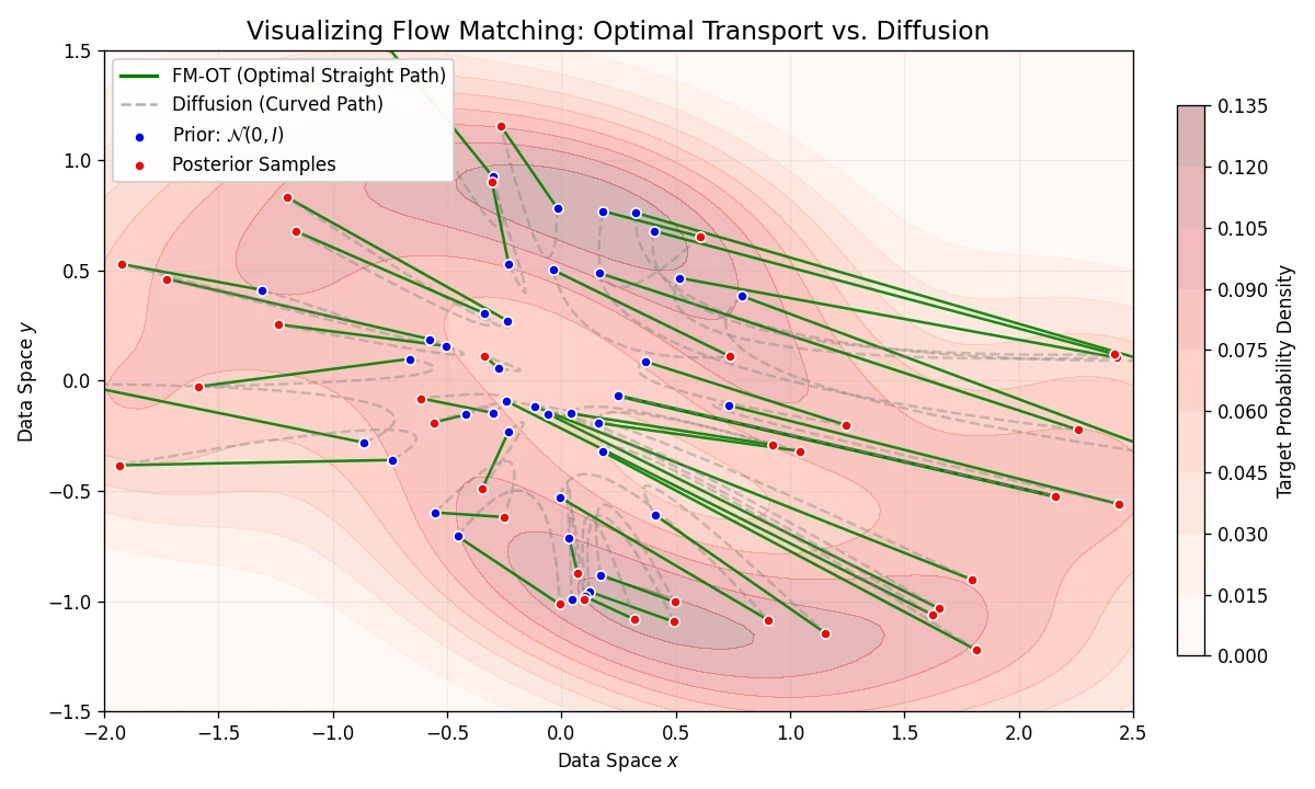
- Goal: To develop an efficient, simulation-free training method for CNFs that supports arbitrary probability paths, specifically allowing for straighter, more efficient trajectories like those from Optimal Transport.
What is the novelty here?
The core novelty is Flow Matching (FM) and specifically the Conditional Flow Matching (CFM) objective.
- Direct Vector Field Regression: The model regresses a target vector field $u_t$ that generates a desired probability path $p_t$.
- Conditional Flow Matching (CFM): The authors prove that regressing the vector field of conditional paths (e.g., $p_t(x|x_1)$ given a single data point) yields the same gradients as regressing the intractable marginal vector field. This bypasses the need to know the marginal score or vector field.
- Optimal Transport Paths: The framework enables the use of Optimal Transport (OT) displacement interpolation for probability paths. OT paths are straight lines with constant speed, leading to faster training and easier sampling.
Concurrent work note: Rectified Flow (Liu et al., 2023) and Stochastic Interpolants (Albergo & Vanden-Eijnden, 2023) were published concurrently at ICLR 2023 with structurally similar contributions under different names. All three independently propose simulation-free training of continuous flows via direct vector field regression; the differences lie in the specific interpolation schemes, theoretical framing, and experimental focus.
What experiments were performed?
- Domains: 2D Checkerboard data, CIFAR-10, and ImageNet at resolutions $32 \times 32$, $64 \times 64$, and $128 \times 128$.
- Task: Unconditional generative modeling (density estimation and sample quality) and conditional super-resolution ($64 \times 64 \to 256 \times 256$).
- Baselines: Compared against Diffusion-based methods on the same architecture (U-Net): DDPM, Score Matching (SM), and ScoreFlow.
- Ablations: Specifically compared FM with Diffusion paths vs. FM with Optimal Transport (OT) paths to isolate the benefit of the training objective vs. the path choice.
What outcomes/conclusions?
- Outperforms diffusion baselines: FM-OT consistently outperforms all diffusion-based methods (DDPM, Score Matching, ScoreFlow) in both Likelihood (NLL) and Sample Quality (FID) across CIFAR-10 and ImageNet, using the same U-Net architecture and training budget. Selected rows from Table 1 (NLL in bits per dimension, BPD; lower is better for all three metrics; “FM w/ OT” and “FM w/ Diffusion” refer to FM trained with OT paths and Diffusion paths respectively):
| Dataset | Method | NLL (BPD) ↓ | FID ↓ | NFE ↓ |
|---|---|---|---|---|
| CIFAR-10 | DDPM | 3.12 | 7.48 | 274 |
| CIFAR-10 | FM w/ OT | 2.99 | 6.35 | 142 |
| ImageNet 64×64 | ScoreFlow | 3.36 | 24.95 | 601 |
| ImageNet 64×64 | FM w/ OT | 3.31 | 14.45 | 138 |
- Training stability: FM with diffusion paths (FM w/ Diffusion) is itself a more stable alternative to diffusion training than DDPM and Score Matching, as shown by training curves in the paper (Figure 5), even before switching to OT paths. The OT path then provides further gains.
- Sampling speed: The straight trajectories of OT paths allow accurate sampling with significantly fewer function evaluations (NFE) compared to diffusion paths.
- Generality: Diffusion is a specific instance of Gaussian probability paths within FM. OT paths are a better-optimized alternative available within the same framework.
- Downstream adoption: Flow matching has been adopted beyond image generation. DynamicFlow uses it as the generative backbone for simultaneously generating ligand molecules and transforming protein pockets, extending flow matching to structure-based drug design.
Reproducibility Details
Data
- Datasets: CIFAR-10, ImageNet ($32 \times 32$, $64 \times 64$, $128 \times 128$).
- Preprocessing:
- Images are center-cropped and resized.
- For $32 \times 32$ and $64 \times 64$, the preprocessing follows Chrabaszcz et al. (2017).
- Data is transformed via $\varphi(y) = 2^7(y+1)$ mapping $[-1, 1]$ pixel values to $[0, 256]$ for BPD computation.
Algorithms
1. Conditional Flow Matching (CFM) Objective
The practical training objective used is the CFM loss, which bypasses intractable marginalization:
$$\mathcal{L}_{CFM}(\theta) = \mathbb{E}_{t, q(x_1), p(x_0)} | v_t(\psi_t(x_0)) - u_t(\psi_t(x_0) | x_1) |^2$$
Where $t \sim \mathcal{U}[0,1]$, $x_1 \sim q(x_1)$ (data), and $x_0 \sim p(x_0)$ (noise).
2. Optimal Transport (OT) Probability Path
The authors recommend the OT path for efficiency.
- Mean/Std Schedule: $\mu_t(x) = t x_1$ and $\sigma_t(x) = 1 - (1 - \sigma_{min})t$.
- Conditional Flow Map: $\psi_t(x) = (1 - (1 - \sigma_{min})t)x + t x_1$.
- Target Vector Field: The closed-form regression target for OT is: $$u_t(x|x_1) = \frac{x_1 - (1 - \sigma_{min})x}{1 - (1 - \sigma_{min})t}$$
3. Sampling
Sampling is performed by solving the ODE $\frac{d}{dt}\phi_t(x) = v_t(\phi_t(x))$ from $t=0$ to $t=1$ using the learned vector field $v_t$.
- Solver:
dopri5(adaptive) is used for robust evaluation. Fixed-step solvers (Euler, Midpoint) are used for low-NFE efficiency tests.
Models
- Architecture: U-Net architecture from Dhariwal & Nichol (2021) is used for all image experiments.
- Toy Data: 5-layer MLP with 512 neurons.
- Hyperparameters:
- Optimizer: Adam ($\beta_1=0.9, \beta_2=0.999$, weight decay=0.0).
- Learning Rate: Polynomial decay or constant (see Table 3 in paper).
- $\sigma_{min}$: Set to a small value (e.g., $1e-5$).
Evaluation
- Metrics:
- NLL (BPD): Computed using the continuous change of variables formula, estimated via the Hutchinson trace estimator to bypass $O(d^3)$ divergence computation.
- FID: Frechet Inception Distance for sample quality.
- NFE: Number of Function Evaluations required by the solver.
- Likelihood Computation: Requires solving an augmented ODE to track the log-density change: $$\frac{d}{dt} \begin{bmatrix} \phi_t(x) \ f(t) \end{bmatrix} = \begin{bmatrix} v_t(\phi_t(x)) \ -\text{div}(v_t(\phi_t(x))) \end{bmatrix}$$
Hardware
- CIFAR-10: 2 GPUs.
- ImageNet-32: 4 GPUs.
- ImageNet-64: 16 GPUs.
- ImageNet-128: 32 GPUs.
- Precision: Full 32-bit for CIFAR/IM-32; 16-bit mixed precision for IM-64/128.
Artifacts
| Artifact | Type | License | Notes |
|---|---|---|---|
| flow_matching (PyTorch library) | Code | CC BY-NC 4.0 | Later official library from Meta; not the original experiment code |
The paper does not release the original training code or model weights used in the experiments. The facebookresearch/flow_matching library was released later as a general-purpose PyTorch implementation of flow matching algorithms. Standard benchmark datasets (CIFAR-10, ImageNet) are publicly available.
Theoretical Notes: Why CFM Works
The paper relies on three key theorems to make training tractable.
Theorem 1 (Marginal Generation):
Marginalizing conditional vector fields $u_t(x|x_1)$ yields the correct marginal vector field $u_t(x)$ that generates the marginal probability path $p_t(x)$.
$$u_t(x) = \int u_t(x|x_1) \frac{p_t(x|x_1)q(x_1)}{p_t(x)} dx_1$$
Understanding the Proof:
To understand why this theorem holds, we have to look at the Continuity Equation, which is the fundamental partial differential equation (PDE) that links a probability density path $p_t$ to a vector field $u_t$.
A vector field $u_t$ is said to “generate” a probability path $p_t$ if and only if they satisfy the continuity equation:
$$\frac{\partial p_t(x)}{\partial t} + \nabla \cdot (p_t(x) u_t(x)) = 0$$
The proof of Theorem 1 relies on substituting the definitions of the marginal path and vector field into this equation to see if they balance out.
Step-by-Step Proof:
Start with the time derivative of the marginal path: We begin by differentiating the marginal probability path $p_t(x)$ with respect to time. By definition, the marginal path is the integral of the conditional paths over the data distribution: $$\frac{\partial p_t(x)}{\partial t} = \frac{\partial}{\partial t} \int p_t(x|x_1) q(x_1) dx_1$$
Swap derivative and integral: Assuming standard regularity conditions (Leibniz Rule), we can move the time derivative inside the integral: $$\frac{\partial p_t(x)}{\partial t} = \int \frac{\partial p_t(x|x_1)}{\partial t} q(x_1) dx_1$$
Apply the Conditional Continuity Equation: This is the critical step. We know that the conditional vector field $u_t(x|x_1)$ generates the conditional path $p_t(x|x_1)$. Therefore, for every single sample $x_1$, the pair satisfies the continuity equation: $$\frac{\partial p_t(x|x_1)}{\partial t} = -\nabla \cdot (p_t(x|x_1) u_t(x|x_1))$$
Substituting this into our integral gives: $$\frac{\partial p_t(x)}{\partial t} = -\int \nabla \cdot (p_t(x|x_1) u_t(x|x_1)) q(x_1) dx_1$$
Pull the Divergence out: Since the divergence operator ($\nabla \cdot$) acts on $x$ and the integral is over $x_1$, we can pull the divergence operator outside the integral (by linearity): $$\frac{\partial p_t(x)}{\partial t} = -\nabla \cdot \left( \int p_t(x|x_1) u_t(x|x_1) q(x_1) dx_1 \right)$$
Match with the Marginal Vector Field Definition: Now, look at the term inside the parentheses. The paper defines the marginal vector field $u_t(x)$ specifically to make this term simpler. Rearranging the definition of $u_t(x)$ provided in the theorem: $$p_t(x) u_t(x) = \int p_t(x|x_1) u_t(x|x_1) q(x_1) dx_1$$
Substitute $p_t(x) u_t(x)$ back into our equation from Step 4: $$\frac{\partial p_t(x)}{\partial t} = -\nabla \cdot (p_t(x) u_t(x))$$
Conclusion: We have just shown that $\frac{\partial p_t(x)}{\partial t} + \nabla \cdot (p_t(x) u_t(x)) = 0$. This is exactly the continuity equation. Because the marginal path and the aggregated marginal vector field satisfy this equation, the vector field is proven to generate the path.
Theorem 2 (Gradient Equivalence):
The intractable Flow Matching objective $\mathcal{L}_{FM}$ (which requires $u_t(x)$) has the same gradients as the tractable Conditional Flow Matching objective $\mathcal{L}_{CFM}$.
$$\nabla_\theta \mathcal{L}_{FM}(\theta) = \nabla_\theta \mathcal{L}_{CFM}(\theta)$$
This allows the model to learn the marginal vector field by only seeing conditional sample paths.
Understanding the Proof:
The reason Theorem 2 holds is that the “Conditional Flow Matching” (CFM) objective is essentially an unbiased estimator of the “Flow Matching” (FM) objective (up to a constant). When we average over all the conditional data points $x_1$, the “cross-term” in the loss function aligns perfectly with the marginal vector field.
1. Expand the Loss Functions
First, let’s look at the squared error in both objectives. Recall that $v_t$ is our neural network (parameterized by $\theta$), $u_t$ is the intractable marginal target, and $u_t(x|x_1)$ is the tractable conditional target.
Expanding the squared norms:
FM Objective: $$\mathcal{L}_{FM}(\theta) = \mathbb{E}_{t, p_t(x)} \left[ |v_t(x)|^2 - 2v_t(x) \cdot u_t(x) + |u_t(x)|^2 \right]$$
CFM Objective: $$\mathcal{L}_{CFM}(\theta) = \mathbb{E}_{t, q(x_1), p_t(x|x_1)} \left[ |v_t(x)|^2 - 2v_t(x) \cdot u_t(x|x_1) + |u_t(x|x_1)|^2 \right]$$
Key Insight: When we take the gradient $\nabla_\theta$, the last term in both equations disappears because the targets ($u_t$) are independent of the network weights $\theta$. We only need to show that the expectations of the first two terms match.
2. Matching the First Term ($|v_t(x)|^2$)
This part is straightforward. The expectation of $|v_t(x)|^2$ is the same in both cases because of how the marginal density $p_t(x)$ is defined.
- FM: averages over $p_t(x)$.
- CFM: averages over $p_t(x|x_1)q(x_1)$.
Since $p_t(x) = \int p_t(x|x_1) q(x_1) dx_1$ (by definition), averaging over the joint distribution is mathematically identical to averaging over the marginal $p_t(x)$.
3. Matching the Cross Term (The “Trick”)
This is the critical part of the proof. We need to show that the interaction between the network and the marginal field equals the interaction between the network and the conditional field.
The Goal: Show $\mathbb{E}_{t, p_t(x)} [v_t(x) \cdot u_t(x)] = \mathbb{E}_{t, q(x_1), p_t(x|x_1)} [v_t(x) \cdot u_t(x|x_1)]$.
The Proof:
Start with the FM cross-term (marginal): $$\mathbb{E}_{t, p_t(x)} [v_t(x) \cdot u_t(x)]$$
Substitute the definition of the marginal vector field $u_t(x)$ derived in Theorem 1: $$u_t(x) = \int u_t(x|x_1) \frac{p_t(x|x_1) q(x_1)}{p_t(x)} dx_1$$
Plug this into the integral. The $p_t(x)$ terms cancel: $$\mathbb{E}_{t, p_t(x)} [v_t(x) \cdot u_t(x)] = \int_t \int_x p_t(x) v_t(x) \cdot \left[ \int_{x_1} u_t(x|x_1) \frac{p_t(x|x_1) q(x_1)}{p_t(x)} dx_1 \right] dx$$
This simplifies to: $$= \int_t \int_x \int_{x_1} v_t(x) \cdot u_t(x|x_1) p_t(x|x_1) q(x_1) dx_1 dx dt$$
This is exactly the definition of the expectation in the CFM objective: $$= \mathbb{E}_{t, q(x_1), p_t(x|x_1)} [v_t(x) \cdot u_t(x|x_1)]$$
Conclusion: Because the expectations of all terms involving $\theta$ are identical, the gradients must be identical.
Intuitively, this works like Denoising Score Matching or Stochastic Gradient Descent: even though each individual conditional vector field $u_t(x|x_1)$ points to a specific data point $x_1$ (which may differ from the true marginal direction), the average of all these pulls equals the true marginal vector field $u_t(x)$.
Theorem 3 (Gaussian Conditional VFs):
For any Gaussian probability path $p_t(x|x_1) = \mathcal{N}(x | \mu_t(x_1), \sigma_t(x_1)^2 I)$, the unique vector field generating it is available in closed form:
$$u_t(x|x_1) = \frac{\sigma’_t(x_1)}{\sigma_t(x_1)}(x - \mu_t(x_1)) + \mu’_t(x_1)$$
This theorem allows explicitly defining targets for both Diffusion (curved) and Optimal Transport (straight) paths.
Understanding the Proof:
The derivation of Theorem 3 comes from the direct relationship between a flow map $\psi_t$ and its generating vector field. Because we chose a specific, simple path (Gaussian), we can invert the flow map to find the vector field in closed form.
1. Define the Flow Map $\psi_t$
We start by defining the conditional probability path as a Gaussian:
$$p_t(x|x_1) = \mathcal{N}(x | \mu_t(x_1), \sigma_t(x_1)^2 I)$$
The simplest way to “push” a standard normal distribution (noise) $p_0 = \mathcal{N}(0, I)$ to this Gaussian is using an affine transformation (scaling and shifting). We define the flow map $\psi_t$ as:
$$\psi_t(x_0) = \sigma_t(x_1) x_0 + \mu_t(x_1)$$
This map takes a noise sample $x_0$ and transforms it into a sample $x$ at time $t$.
2. The Definition of a Generating Vector Field
By definition, a vector field $u_t$ generates a flow $\psi_t$ if the vector field describes the instantaneous velocity of the flow at any point. Mathematically:
$$u_t(\psi_t(x_0)) = \frac{d}{dt}\psi_t(x_0)$$
Let $x = \psi_t(x_0)$ be the position of the particle at time $t$. We want to find $u_t(x)$.
3. Invert the Flow Map
To find $u_t(x)$, we must express the equation in terms of $x$ rather than $x_0$. Since our flow map is a simple affine transformation (multiply and add), it is easily invertible (assuming $\sigma_t(x_1) \neq 0$):
$$x_0 = \frac{x - \mu_t(x_1)}{\sigma_t(x_1)}$$
We will call this inverse map $\psi_t^{-1}(x)$.
4. Differentiate the Flow Map
Now we calculate the left side of our definition equation (velocity): $\frac{d}{dt}\psi_t(x_0)$.
Taking the time derivative of $\psi_t(x_0) = \sigma_t(x_1) x_0 + \mu_t(x_1)$:
$$\frac{d}{dt}\psi_t(x_0) = \sigma’_t(x_1) x_0 + \mu’_t(x_1)$$
(Note: $\sigma’_t$ and $\mu’_t$ denote time derivatives).
5. Substitute and Solve
Now we combine everything. We know $u_t(\psi_t(x_0)) = \frac{d}{dt}\psi_t(x_0)$.
Substitute the result from Step 4 into this equation:
$$u_t(\psi_t(x_0)) = \sigma’_t(x_1) x_0 + \mu’_t(x_1)$$
This expresses the vector field in terms of the initial point $x_0$. We must express it in terms of the current point $x$. So, we plug in the inverse formula for $x_0$ derived in Step 3:
$$u_t(x|x_1) = \sigma’_t(x_1) \frac{x - \mu_t(x_1)}{\sigma_t(x_1)} + \mu’_t(x_1)$$
Rearranging terms gives the final closed form:
$$u_t(x|x_1) = \frac{\sigma’_t(x_1)}{\sigma_t(x_1)}(x - \mu_t(x_1)) + \mu’_t(x_1)$$
Why is this useful?
This formula means that as long as you can define a mean schedule $\mu_t(x_1)$ and a standard deviation schedule $\sigma_t(x_1)$ (which is easy to do for both Diffusion and Optimal Transport), you immediately get the exact vector field target $u_t(x|x_1)$ needed to train your neural network, bypassing complex ODE solving or score matching approximations.
Paper Information
Citation: Lipman, Y., Chen, R. T. Q., Ben-Hamu, H., Nickel, M., & Le, M. (2023). Flow Matching for Generative Modeling. International Conference on Learning Representations (ICLR).
Publication: ICLR 2023
@inproceedings{lipmanFlowMatchingGenerative2023,
  title = {Flow Matching for Generative Modeling},
  author = {Lipman, Yaron and Chen, Ricky T. Q. and Ben-Hamu, Heli and Nickel, Maximilian and Le, Matt},
  booktitle = {International Conference on Learning Representations},
  year = {2023}
}
Additional Resources: