What kind of paper is this?
This is a method paper that introduces a training approach for Variational Autoencoders (VAEs) to address fundamental limitations in their generative quality through improved prior learning.
What is the motivation?
The work is motivated by a critical limitation in Variational Autoencoders known as the “prior hole” problem, where the prior distribution p(z) fails to match the aggregate approximate posterior q(z). This mismatch leads to areas in the latent space with high density under the prior that don’t map to realistic data samples, resulting in poor generative quality compared to GANs and other generative models.
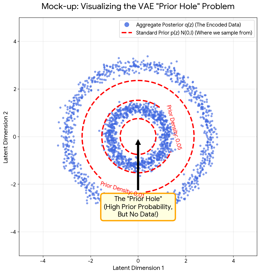
 with an empty center, while the standard Gaussian prior p(z) has highest density at the center where no data exists")
The figure above illustrates this mismatch. The blue dots represent where a trained encoder actually places data in the latent space (the aggregate posterior $q(z)$), which often forms complex, non-Gaussian shapes. The red dashed contours show the standard Gaussian prior $p(z) = \mathcal{N}(0, I)$, which assumes data is centered at the origin. When generating new samples, we draw from this prior, making it likely to sample from the empty “hole” where the decoder has never seen training data, producing unrealistic outputs.
A natural question arises: the prior $p(z)$ is used for sampling at inference time, so why does learning a better prior also improve likelihood (NLL)? The answer lies in the VAE objective. VAEs maximize the Evidence Lower Bound (ELBO):
$$ \log p(x) \geq \mathcal{L}_{\text{ELBO}}(x) = \underbrace{\mathbb{E}_{q(z|x)}[\log p(x|z)]}_{\text{Reconstruction}} - \underbrace{\text{KL}(q(z|x) \parallel p(z))}_{\text{Regularization}} $$
The KL divergence term penalizes the mismatch between each data point’s approximate posterior $q(z|x)$ and the prior $p(z)$. When the prior is a simple Gaussian but the aggregate posterior forms a complex shape (as in the figure above), this KL term remains unnecessarily high for every data point.
By replacing the simple prior with a learned $p_{\text{NCP}}(z)$ that matches the aggregate posterior, the KL penalty decreases, tightening the ELBO and improving NLL. The learned prior thus provides a unified solution: better likelihood during training (tighter bound) and better sampling at inference (no “holes”).
The OpenReview discussion contains a significant theoretical debate regarding the paper’s core premise. Reviewers argued that the “prior hole” problem is actually a failure of the posterior to match the prior, or a failure of the encoder. The authors defended their approach by noting that even with a perfect posterior, a simple Normal prior might fail because the decoder lacks capacity to map a simple distribution to complex data without dropping modes. This justifies fixing the prior by making it learned and complex.
What is the novelty here?
The authors propose an energy-based model (EBM) prior that is trained using Noise Contrastive Estimation (NCE), which they term a Noise Contrastive Prior (NCP). The key innovations are:
- Two-Stage Training Process: First, a standard VAE is trained with a simple base prior. Then, the VAE weights are frozen and a binary classifier learns to distinguish between samples from the aggregate posterior q(z) and the base prior p(z).
- Reweighting Strategy: The core idea is to reweight a base prior distribution p(z) with a learned reweighting factor r(z) to make the resulting prior $p_{\text{NCP}}(z)$ better match the aggregate posterior q(z).
- NCE for EBM Training: The method frames EBM training as a binary classification task to avoid computationally expensive MCMC sampling.
- Scalability to Hierarchical Models: For hierarchical VAEs with multiple latent groups, the NCP approach can be applied independently and in parallel to each group’s conditional prior.
What experiments were performed?
The method was evaluated on several standard image generation benchmarks:
- MNIST (dynamically binarized): Likelihood evaluation on a controlled, small-latent-space task
- CIFAR-10: Standard computer vision benchmark for generative modeling
- CelebA 64x64: Applied to both standard VAE architectures and more advanced VAEs with GMM priors (RAE model)
- CelebA HQ 256x256: High-resolution face generation task
The hierarchical NVAE models used 30 latent groups for CIFAR-10 and CelebA-64, 20 groups for CelebA-HQ-256, and 10 groups of $4 \times 4$ latent variables for MNIST (deliberately small to enable reliable partition function estimation). The experiments compared FID scores, likelihood metrics, and qualitative sample quality between baseline VAEs and NCP-enhanced versions, with particular focus on hierarchical VAEs (NVAE).
What outcomes/conclusions?
The proposed NCP method demonstrated improvements in generative quality across evaluated datasets, with modest gains on standard VAEs and particularly large gains on hierarchical models like NVAE:
- CelebA-64: NCP improved FID scores from 48.12 to 41.28 for standard VAEs, and from 40.95 to 39.00 for RAE models with GMM priors.
- Hierarchical Models (NVAE): The impact was particularly pronounced on hierarchical VAEs:
- CIFAR-10: FID improved from 51.71 to 24.08
- CelebA-64: FID improved from 13.48 to 5.25, making it competitive with GANs
- CelebA HQ 256x256: FID reduced from 40.26 to 24.79
- Likelihood Performance: On MNIST, NCP-VAE achieved 78.10 nats NLL vs. baseline NVAE’s 78.67 nats
On CIFAR-10 and CelebA-HQ-256, the concurrent VAEBM method (which forms an EBM on the data space rather than the latent space) outperforms NCP-VAE. However, the authors argue the two approaches are complementary: NCP-VAE targets the latent space while VAEBM operates in data space, and combining them could yield further gains. NCP-VAE also has the advantage of applicability to discrete data (e.g., binarized MNIST) and simpler setup since it only requires training binary classifiers rather than MCMC-based training and sampling.
The key conclusions are that two-stage training with noise contrastive estimation provides an effective framework for learning expressive energy-based priors that addresses the prior hole problem while scaling efficiently to hierarchical models.
Reproducibility Details
| Artifact | Type | License | Notes |
|---|---|---|---|
| Code (Google Drive) | Code | Unknown | Official implementation; hosted on Google Drive (may become inaccessible) |
| OpenReview | Other | N/A | Reviews, author responses, and supplementary material |
Algorithms
The Reweighting Mechanism
The core innovation is defining the NCP prior as $p_{\text{NCP}}(z) \propto p(z)r(z)$. The reweighting factor $r(z)$ is derived from the binary classifier $D(z)$ using the likelihood ratio trick:
$$ r(z) \approx \frac{D(z)}{1 - D(z)} $$
Here, $D(z)$ is the sigmoid output of the trained discriminator, representing the probability that sample $z$ came from the aggregate posterior $q(z)$ (“real”). For an optimal discriminator $D^*(z)$, this ratio exactly equals $\frac{q(z)}{p(z)}$, allowing the model to approximate the density ratio without explicit density estimation.
 the complex bimodal aggregate posterior, p(z) the simple Gaussian prior, and r(z) the learned reweighting factor that transforms p(z) to match q(z)")
Hierarchical Architecture Strategy
For hierarchical models (like NVAE), the method trains $K$ binary classifiers in parallel (one for each latent group). Crucially, to ensure efficiency, the classifiers reuse the context feature $c(z_{<k})$ extracted by the frozen VAE’s prior network. This architectural choice provides significant computational savings.
Test-Time Sampling (Inference)
Since $p_{\text{NCP}}(z)$ is an energy-based model, direct sampling is impossible. The paper employs two methods to generate samples:
- Sampling-Importance-Resampling (SIR): Used for most results. It draws $M$ samples (e.g., $M=5000$) from the base prior $p(z)$ and resamples them based on weights $w^{(m)} = r(z^{(m)})$.
- Langevin Dynamics (LD): An iterative refinement method using the gradient of the energy function $E(z) = -\log r(z) - \log p(z)$.
Models
Decoder Architecture
For RGB datasets (CIFAR-10, CelebA), the output likelihood must be changed from Discretized Logistic (standard NVAE) to a Normal distribution. The authors note this change alone led to “significant improvements in the base model performance.” Using the standard NVAE decoder will result in a weaker baseline than reported.
Discriminator Architecture
The binary classifier uses a ResNet-style architecture with Squeeze-and-Excitation (SE) blocks:
- Activation: Swish
- Normalization: Batch Normalization
- Optimization: Adam with Cosine Annealing (learning rate: $10^{-3} \to 10^{-7}$)
The SE blocks help the model focus on channel-wise feature recalibration, which is important for distinguishing subtle differences between prior and aggregate posterior in high-dimensional latent spaces.
Hardware
The main paper is vague on training time, but the OpenReview rebuttal explicitly lists hardware costs:
- Hardware: NVIDIA Tesla V100 (32GB) GPUs
- Per-Discriminator Training: ~13 hours for 100 epochs
- Parallelization: Because latent groups are independent, all discriminators can train in parallel
- Total Cost (CelebA-64): ~8.1 GPU-days
- Comparison: The authors argue this is efficient compared to VDVAE, which requires ~560 GPU-days
Evaluation
Inference Speed vs. Quality Trade-off
Reviewers flagged that SIR sampling can be prohibitively slow. The authors clarified the exact trade-off:
| Proposal Samples ($M$) | Time per Image | FID (CelebA-64) |
|---|---|---|
| 5,000 (paper default) | ~10.11 seconds | 5.25 |
| 500 (practical) | ~1.25 seconds | 6.76 |
The quality gain from 500 to 5,000 samples is modest (FID difference of 1.51) while inference time increases roughly 8x, suggesting $M=500$ may be a practical default.
Hyperparameters
- FID Calculation: 50,000 samples
- SIR Proposals: 5,000 samples (paper default) or 500 (practical)
- MNIST: Dynamically binarized version used for likelihood evaluation
- Optimizers: The study largely adopts hyperparameters from baseline papers (e.g., Lawson et al. for MNIST, Ghosh et al. for RAE)
Debugging Benchmark: 25-Gaussians
The supplement provides a toy experiment ideal for verifying a new implementation before running on expensive image datasets:
- Setup: Synthetic dataset of 25 2D-Gaussians arranged on a grid
- Target NLL: ~-0.954 nats (NCP) vs. ~-2.753 nats (Vanilla VAE)
- Success Criterion: Samples should avoid low-density regions between grid points. A standard VAE will generate samples in these “prior holes,” while a working NCP implementation should cleanly remove these artifacts.
Implementation Warnings
- SIR Failure Mode: If the learned prior $p_{\text{NCP}}$ deviates too far from the base prior, SIR sampling collapses (low effective sample size). The paper shows a strong correlation between the NCE classification loss and the effective sample size (Fig. 5(b)), indicating that SIR reliability depends on how well the base prior matches the aggregate posterior.
- Temperature Scaling: The qualitative images in the paper use reduced temperature for improved visual sharpness (Section 5.3). The FID tables do not specify a temperature, so results may or may not use $T=1.0$.
Data
The method was evaluated on several standard image generation benchmarks:
- MNIST (dynamically binarized): Likelihood evaluation on a controlled, small-latent-space task
- CIFAR-10: Standard computer vision benchmark for generative modeling (32x32 RGB images)
- CelebA 64x64: Face generation task with moderate resolution
- CelebA HQ 256x256: High-resolution face generation task
All datasets use standard train/test splits from the computer vision literature.
Additional Metrics
Beyond FID and NLL, the paper uses:
- Effective Sample Size (ESS): Validates reliability of the SIR sampling procedure
- Maximum Mean Discrepancy (MMD): Measures distance between aggregate posterior and NCP prior distributions
Paper Information
Citation: Aneja, J., Schwing, A. G., Kautz, J., & Vahdat, A. (2021). A contrastive learning approach for training variational autoencoder priors. Advances in Neural Information Processing Systems, 34, 29604-29616. https://proceedings.neurips.cc/paper/2021/hash/0496604c1d80f66fbeb963c12e570a26-Abstract.html
Publication: NeurIPS 2021
@inproceedings{aneja2021contrastive,
  title={A Contrastive Learning Approach for Training Variational Autoencoder Priors},
  author={Aneja, Jyoti and Schwing, Alexander G and Kautz, Jan and Vahdat, Arash},
  booktitle={Advances in Neural Information Processing Systems},
  volume={34},
  pages={29604--29616},
  year={2021}
}
Additional Resources:
- OpenReview Discussion
- Code Repository (Google Drive; link may become inaccessible over time)