What kind of paper is this?
This is a Method paper that introduces a generative mechanism (the VAE) and an optimization technique (the reparameterization trick), with formal theoretical derivation. The method, called the Auto-Encoding VB (AEVB) algorithm, leads to what we now know as the variational auto-encoder (VAE) when neural networks are used as the recognition model.
What is the motivation?
The authors address two central intractabilities in directed probabilistic models with continuous latent variables:

Intractable Posteriors: In models with continuous latent variables (like those with non-linear hidden layers), the true posterior $p_{\theta}(z|x)$ cannot be calculated analytically, preventing the use of standard EM algorithms.
Large Datasets: Sampling-based solutions like Monte Carlo EM (MCEM) require expensive sampling loops per datapoint. This makes them too slow for large datasets where batch optimization is too costly and efficient minibatch updates are required.
What is the novelty here?
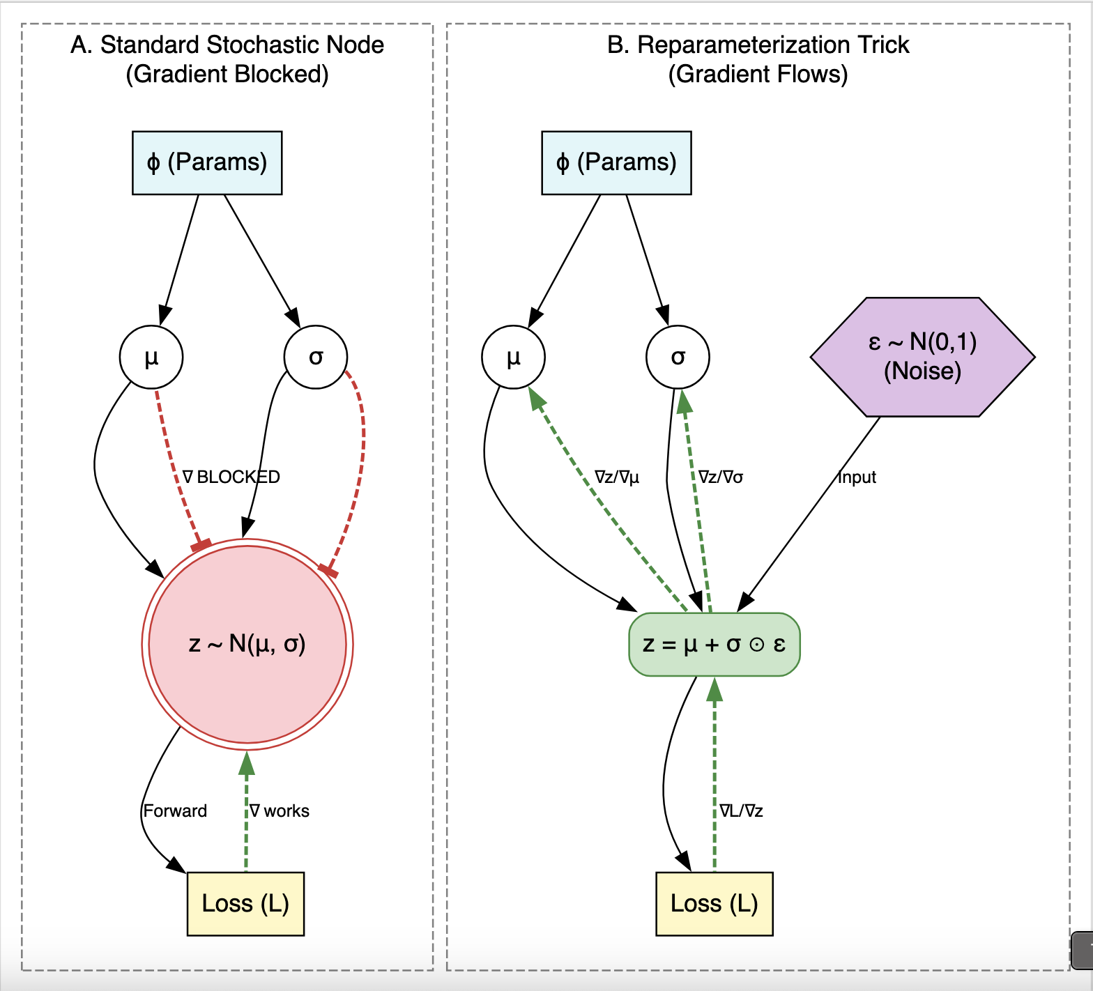
The Reparameterization Trick (SGVB Estimator)
The core innovation is the Stochastic Gradient Variational Bayes (SGVB) estimator. The authors solve the high variance of standard gradient estimation by “reparameterizing” the random variable $\tilde{z}$.
They express $z$ as a deterministic function of the input $x$ and an auxiliary noise variable $\epsilon$:
$$\tilde{z} = g_{\phi}(\epsilon, x) \quad \text{with} \quad \epsilon \sim p(\epsilon)$$

- Mechanism: For a Gaussian posterior, $z = \mu + \sigma \odot \epsilon$ where $\epsilon \sim \mathcal{N}(0, I)$.
- Impact: This makes the Monte Carlo estimate differentiable with respect to the variational parameters $\phi$, allowing the variational lower bound to be optimized via standard stochastic gradient ascent (like SGD or Adagrad).
The AEVB Algorithm (The VAE)
The Auto-Encoding VB (AEVB) algorithm amortizes inference by learning a global recognition model (encoder) $q_{\phi}(z|x)$ jointly with the generative model (decoder) $p_{\theta}(x|z)$.
Objective Function: Maximize the variational lower bound $\mathcal{L}(\theta, \phi; x^{(i)})$:
$$\mathcal{L} \simeq -D_{KL}(q_\phi(z|x^{(i)}) | p_\theta(z)) + \frac{1}{L} \sum_{l=1}^L \log p_\theta(x^{(i)}|z^{(i,l)})$$
- First Term (Regularizer): Forces the approximate posterior to match the prior (integrated analytically for Gaussians).
- Second Term (Reconstruction Error): The expected negative reconstruction error (estimated via sampling).
This mirrors the standard auto-encoder objective, adding a variational regularizer.
What experiments were performed?
The method was benchmarked against the Wake-Sleep algorithm and Monte Carlo EM (MCEM) using the MNIST (digits) and Frey Face (continuous faces) datasets.
What outcomes/conclusions?
Efficiency: AEVB converged faster and reached a better lower bound than Wake-Sleep (Figure 2). It scaled efficiently to the full MNIST dataset. MCEM’s per-datapoint sampling cost made it impractical at full dataset scale, so comparisons were limited to small subsets (Figure 3).
Regularization: The KL-divergence term provided a regularizing effect, preventing overfitting while increasing latent dimensions ($N_z$).
Manifold Learning: The model successfully learned smooth 2D latent manifolds (visualized in Appendix A), grouping similar digits/faces together.
Reproducibility Details
Data
Evaluation Data: For the marginal likelihood comparison (Figure 3), the paper used MNIST with $N_{\text{train}} = 100$ and $N_{\text{train}} = 5000$ to compare data efficiency (marginal log-likelihood vs. training samples seen) across algorithms. A smaller network (100 hidden units, 3 latent variables) was used for this comparison because the marginal likelihood estimator only works reliably in low-dimensional latent spaces.
Algorithms
- Algorithm: Stochastic gradient ascent with Adagrad (global stepsizes chosen from ${0.01, 0.02, 0.1}$).
- Regularization: The objective included a weight decay term corresponding to a prior $p(\theta)=\mathcal{N}(0,I)$.
- Minibatches: Size $M=100$ with $L=1$ sample per datapoint.
- Initialization: Parameters sampled from $\mathcal{N}(0, 0.01)$.
Models
The original VAE used simple Multi-Layered Perceptrons (MLPs):
- Symmetry: The encoder and decoder were symmetric, having an equal number of hidden units.
- Hidden Units: 500 units for MNIST, 200 for Frey Face (to prevent overfitting on the smaller dataset).
- Activations: Tanh activation functions for the hidden layers.
- Latent Space: Experimented with $N_z$ ranging from 2 to 200.
- Outputs:
- MNIST: Bernoulli MLP (sigmoid output).
- Frey Face: Gaussian MLP, with means constrained to $(0,1)$ via sigmoid.
- Encoder Architecture: For the Gaussian encoder, the mean $\mu$ and log-variance $\log(\sigma^2)$ are linear outputs from the shared hidden layer (they share the hidden layer weights and have separate output weights).
- Log-Variance: The encoder predicted $\log(\sigma^2)$ for numerical stability.
Evaluation
The paper distinguishes between two metrics:
- Variational Lower Bound: Used as the training objective (what the model optimizes).
- Marginal Likelihood: Used for final evaluation (Figure 3). The true marginal likelihood $p_\theta(x)$ was estimated using an Importance Sampling estimator constructed from samples drawn via Hybrid Monte Carlo (HMC), as detailed in Appendix D. This estimator uses: $p_{\theta}(x^{(i)}) \simeq (\frac{1}{L}\sum \frac{q(z)}{p(z)p(x|z)})^{-1}$.
This distinction is critical: the training metric (lower bound) differs from the evaluation metric (estimated marginal likelihood).
Hardware
- Hardware: Trained on a standard Intel Xeon CPU (approx. 40 GFLOPS); no GPUs were used.
- Training Time: Approximately 20-40 minutes per million training samples.
Key Implementation Details from Appendices
- Appendix A: Visualizations of 2D latent manifolds learned for MNIST and Frey Face datasets.
- Appendix B: Closed-form solution for the KL divergence of two Gaussians, essential for implementing the efficient version of the estimator (Equation 10).
- Appendix C: Exact MLP equations, including the use of tanh hidden layers and specific output layers for Bernoulli vs. Gaussian data. Includes specifications for Bernoulli MLPs (binary data) and Gaussian MLPs (real-valued data).
- Appendix D: Marginal likelihood estimation protocol using Hybrid Monte Carlo (HMC) and importance sampling for evaluation (Figure 3).
Paper Information
Citation: Diederik P. Kingma and Max Welling. “Auto-Encoding Variational Bayes.” arXiv:1312.6114 [stat.ML], 2013. https://doi.org/10.48550/arXiv.1312.6114
Publication: ICLR 2014 (arXiv preprint December 2013)
@misc{kingma2022autoencodingvariationalbayes,
      title={Auto-Encoding Variational Bayes},
      author={Diederik P Kingma and Max Welling},
      year={2013},
      eprint={1312.6114},
      archivePrefix={arXiv},
      primaryClass={stat.ML},
      url={https://arxiv.org/abs/1312.6114},
}
Additional Resources:
- Wikipedia: Variational Autoencoder - General overview
- OpenReview - Original peer review with author responses
- Modern VAE in PyTorch - Implementation tutorial on this site