Paper Information
Citation: Oldenhof, M., Arany, A., Moreau, Y., & Simm, J. (2020). ChemGrapher: Optical Graph Recognition of Chemical Compounds by Deep Learning. Journal of Chemical Information and Modeling, 60(10), 4506-4517. https://doi.org/10.1021/acs.jcim.0c00459
Publication: Journal of Chemical Information and Modeling 2020 (arXiv preprint Feb 2020)
Additional Resources:
Classifying the Methodology
This is a Method paper. It proposes a novel deep learning architecture and a specific graph-reconstruction algorithm to solve the problem of Optical Chemical Structure Recognition (OCSR). It validates this method by comparing it against the existing standard tool (OSRA), demonstrating superior performance on specific technical challenges like stereochemistry.
The OCR Stereochemistry Challenge
Chemical knowledge is frequently locked in static images within scientific publications. Extracting this structure into machine-readable formats (graphs, SMILES) is essential for drug discovery and database querying. Existing tools, such as OSRA, rely on optical character recognition (OCR) and expert systems or hand-coded rules. These tools struggle with bond multiplicity and stereochemical information, often missing atoms or misinterpreting 3D cues (wedges and dashes). A machine learning approach allows for improvement via data scaling.
Decoupled Semantic Segmentation and Classification Pipeline
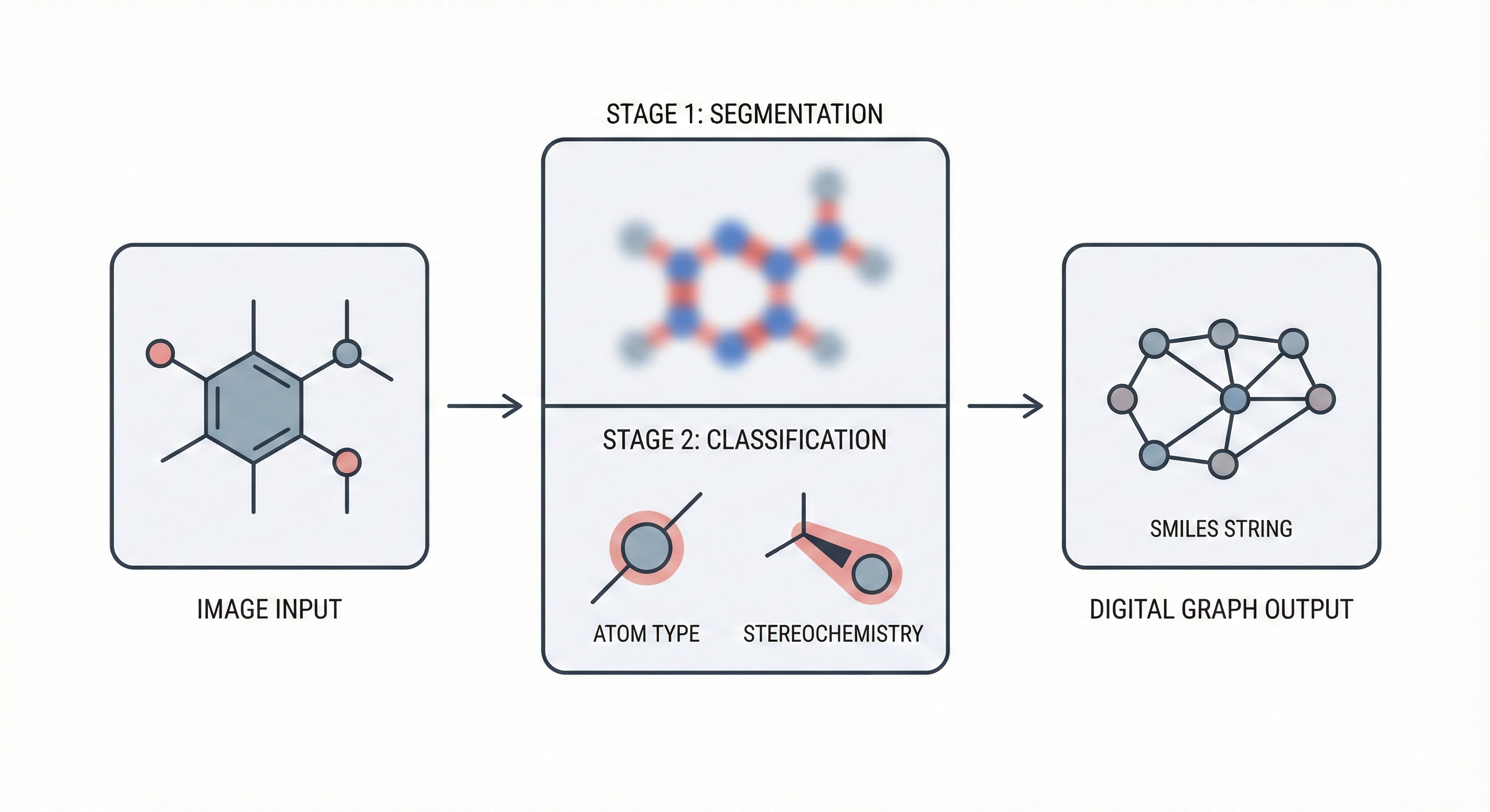
The core novelty is the segmentation-classification pipeline which decouples object detection from type assignment:
- Semantic Segmentation: The model first predicts pixel-wise maps for atoms, bonds, and charges using a modified U-Net/dilated convolution architecture.
- Graph Building Algorithm: A specific algorithm iterates over the segmentation maps to generate candidate locations for atoms and bonds.
- Refinement via Classification: Dedicated classification networks take cutouts of the original image combined with the segmentation mask to verify and classify each candidate (e.g., distinguishing a single bond from a double bond, or a wedge from a dash).
Additionally, the authors developed a novel method for synthetic data generation by modifying the source code of RDKit to output pixel-wise labels during the image drawing process. This solves the lack of labeled training data.
Evaluating Synthetics and Benchmarks
- Synthetic Benchmarking: The authors generated test sets in 3 different stylistic variations. For each style, they tested on both stereo (complex 3D information) and non-stereo compounds.
- Baseline Comparison: They compared the error rates of ChemGrapher against OSRA (Optical Structure Recognition Application).
- Ablation Study: They analyzed the F1 scores of the segmentation networks versus the classification networks independently to understand where errors propagated.
- Real-world Case Study: They manually curated 61 images cut from journal articles to test performance on real, non-synthetic data.
Advancements Over OSRA
- Superior Accuracy: ChemGrapher consistently achieved lower error rates than OSRA across all synthetic styles, particularly for stereochemical information (wedge and dash bonds).
- Component Performance: The classification networks showed significantly higher F1 scores than the segmentation networks. This suggests the two-stage approach allows the classifier to correct segmentation noise.
- Real-world Viability: In the manual case study, ChemGrapher correctly predicted 46 of 61 images, compared to 42 of 61 for OSRA.
- Limitations: The model struggles with thick bond lines and non-carbon atom labels in real-world images due to the bias in the synthetic training data.
Reproducibility Details
Data
The authors created a custom synthetic dataset using ChEMBL and RDKit, as no pixel-wise labeled dataset existed.
| Purpose | Dataset | Size | Notes |
|---|---|---|---|
| Source | ChEMBL | 1.9M | Split into training pool (1.5M), val/train pool (300K), and test pools (35K each). |
| Segmentation Train | Synthetic | ~114K | Sampled from ChEMBL pool such that every atom type appears in >1000 compounds. |
| Labels | Pixel-wise | N/A | Generated by modifying RDKit source code to output label masks (atom type, bond type, charge) during drawing. |
| Candidates | Cutouts | ~27K (Atom) ~55K (Bond) | Generated from the validation pool for training the classification networks. |
Algorithms
Algorithm 1: Graph Building
- Segment: Apply segmentation network $s(x)$ to get maps $S^a$ (atoms), $S^b$ (bonds), $S^c$ (charges).
- Atom Candidates: Identify candidate blobs in $S^a$.
- Classify Atoms: For each candidate, crop the input image and segmentation map. Feed to $c_A$ and $c_C$ to predict Atom Type and Charge. Add to Vertex set $V$ if valid.
- Bond Candidates: Generate all pairs of nodes in $V$ within $2 \times$ bond length distance.
- Classify Bonds: For each pair, create a candidate mask (two rectangles meeting in the middle to encode directionality). Feed to $c_B$ to predict Bond Type (single, double, wedge, etc.). Add to Edge set $E$.
Models
The pipeline uses four distinct Convolutional Neural Networks (CNNs).
1. Semantic Segmentation Network ($s$)
- Architecture: 8-layer fully convolutional network (Dense Prediction Convolutional Network).
- Kernels: $3\times3$ for all layers.
- Dilation: Uses dilated convolutions to expand receptive field without losing resolution. Dilations: 1, 2, 4, 8, 8, 4, 2, 1.
- Input: Binary B/W image.
- Output: Multi-channel probability maps for Atom Types ($S^a$), Bond Types ($S^b$), and Charges ($S^c$).
2. Classification Networks ($c_A, c_B, c_C$)
- Purpose: Refines predictions on small image patches.
- Architecture: 5 convolutional layers followed by a MaxPool and 2 Fully Connected layers.
- Layer 1: Depthwise separable convolution.
- Layers 2-4: Dilated convolutions (factors 2, 4, 8).
- Layer 5: Standard convolution + MaxPool ($124 \x124$).
- Inputs:
- Crop of the binary image ($x^{cut}$).
- Crop of the segmentation map ($S^{cut}$).
- “Highlight” mask ($h_L$) indicating the specific candidate location (e.g., a dot for atoms, two rectangles for bonds).
Evaluation
- Metric: F1 Score for individual network performance (segmentation pixels and classification accuracy).
- Metric: Error Rate (percentage of incorrect graphs) for overall system. A graph is “incorrect” if there is at least one mistake in atoms or bonds.
- Baselines: Compared against OSRA (v2.1.0 implied by context of standard tools).
Hardware
- GPU: Training and inference performed on a single NVIDIA Titan Xp.
Citation
@article{oldenhof2020chemgrapher,
  title={ChemGrapher: Optical Graph Recognition of Chemical Compounds by Deep Learning},
  author={Oldenhof, Martijn and Arany, Adam and Moreau, Yves and Simm, Jaak},
  journal={Journal of Chemical Information and Modeling},
  volume={60},
  number={10},
  pages={4506--4517},
  year={2020},
  publisher={ACS Publications},
  doi={10.1021/acs.jcim.0c00459}
}