Paper Typology and Contribution
This is a Method paper. It challenges the atom-centric paradigm of molecular representation learning by proposing a novel framework that models the continuous 3D space surrounding atoms. The core contribution is SpaceFormer, a Transformer-based architecture that discretizes molecular space into grids to capture physical phenomena (electron density, electromagnetic fields) often missed by traditional point-cloud models.
The Physical Intuition: Modeling “Empty” Space
The Gap: Prior 3D molecular representation models, such as Uni-Mol, treat molecules as discrete sets of atoms, essentially point clouds in 3D space. However, from a quantum physics perspective, the “empty” space between atoms is far from empty. It is permeated by electron density distributions and electromagnetic fields that determine molecular properties.
The Hypothesis: Explicitly modeling this continuous 3D space alongside discrete atom positions yields superior representations for downstream tasks, particularly for computational properties that depend on electronic structure, such as HOMO/LUMO energies and energy gaps.
A Surprising Observation: Virtual Points Improve Representations
Before proposing SpaceFormer, the authors present a simple yet revealing experiment. They augment Uni-Mol by adding randomly sampled virtual points (VPs) from the 3D space within the circumscribed cuboid of each molecule. These VPs carry no chemical information whatsoever: they are purely random noise points.
The result is surprising: adding just 10 random VPs already yields a noticeable improvement in validation loss. The improvement remains consistent and gradually increases as the number of VPs grows, eventually reaching a plateau. This observation holds across downstream tasks as well, with Uni-Mol + VPs improving on several quantum property predictions (LUMO, E1-CC2, E2-CC2) compared to vanilla Uni-Mol.
The implication is that even uninformative spatial context helps the model learn better representations, motivating a principled framework for modeling the full 3D molecular space.
SpaceFormer: Voxelization and 3D Positional Encodings
The key innovation is treating the molecular representation problem as 3D space modeling. SpaceFormer follows these core steps:
- Voxelizes the entire 3D space into a grid with cells of $0.49\text{\AA}$ (based on O-H bond length to ensure at most one atom per cell).
- Uses adaptive multi-resolution grids to efficiently handle empty space, keeping it fine-grained near atoms and coarse-grained far away.
- Applies Transformers to 3D spatial tokens with custom positional encodings that achieve linear complexity.
Specifically, the model utilizes two forms of 3D Positional Encoding:
3D Directional PE (RoPE Extension) They extend Rotary Positional Encoding (RoPE) to 3D continuous space by splitting the Query and Key vectors into three blocks (one for each spatial axis). The directional attention mechanism takes the form:
$$ \begin{aligned} \mathbf{q}_{i}^{\top} \mathbf{k}_{j} = \sum_{s=1}^{3} \mathbf{q}_{i,s}^{\top} \mathbf{R}(c_{j,s} - c_{i,s}) \mathbf{k}_{j,s} \end{aligned} $$
3D Distance PE (RFF Approximation) To compute invariant geometric distance without incurring quadratic memory overhead, they use Random Fourier Features (RFF) to approximate a Gaussian kernel of pairwise distances:
$$ \begin{aligned} \exp \left( - \frac{| \mathbf{c}_i - \mathbf{c}_j |_2^2}{2\sigma^2} \right) &\approx z(\mathbf{c}_i)^\top z(\mathbf{c}_j) \\ z(\mathbf{c}_i) &= \sqrt{\frac{2}{d}} \cos(\sigma^{-1} \mathbf{c}_i^\top \boldsymbol{\omega} + \mathbf{b}) \end{aligned} $$
This approach enables the model to natively encode complex field-like phenomena without computing exhaustive $O(N^2)$ distance matrices.
Experimental Setup and Downstream Tasks
Pretraining Data: 19 million unlabeled molecules from the same dataset used by Uni-Mol.
Downstream Benchmarks: The authors propose a new benchmark of 15 tasks, motivated by known limitations of MoleculeNet: invalid structures, inconsistent chemical representations, data curation errors, and an inability to adequately distinguish model performance. The tasks split into two categories:
Computational Properties (Quantum Mechanics)
- Subsets of GDB-17 (HOMO, LUMO, GAP energy prediction, 20K samples; E1-CC2, E2-CC2, f1-CC2, f2-CC2, 21.7K samples)
- Cata-condensed polybenzenoid hydrocarbons (Dipole moment, adiabatic ionization potential, D3 dispersion correction, 8,678 samples)
- Metric: Mean Absolute Error (MAE)
Experimental Properties (Pharma/Bio)
- MoleculeNet tasks (BBBP, BACE for drug discovery)
- Biogen ADME tasks (HLM, MME, Solubility)
- Metrics: AUC for classification, MAE for regression
Splitting Strategy: All datasets use 8:1:1 train/validation/test ratio with scaffold splitting to test out-of-distribution generalization.
Training Setup:
- Objective: Masked Auto-Encoder (MAE) with 30% random masking. Model predicts whether a cell contains an atom, and if so, regresses both atom type and precise offset position.
- Hardware: ~50 hours on 8 NVIDIA A100 GPUs
- Optimizer: Adam ($\beta_1=0.9, \beta_2=0.99$)
- Learning Rate: Peak 1e-4 with linear decay and 0.01 warmup ratio
- Batch Size: 128
- Total Updates: 1 million
Baseline Comparisons: GROVER (2D graph-based MPR), GEM (2D graph enhanced with 3D information), 3D Infomax (GNN with 3D information), Uni-Mol (3D MPR, primary baseline using the same pretraining dataset), and Mol-AE (extends Uni-Mol with atom-based MAE pretraining).
Results and Analysis
Strong Contextual Performance: SpaceFormer ranked 1st in 10 of 15 tasks and in the top 2 for 14 of 15 tasks. It surpassed the runner-up models by approximately 20% on quantum property tasks (HOMO, LUMO, GAP, E1-CC2, Dipmom), validating that modeling non-atom space captures electronic structure better than atom-only regimes.
Key Results on Quantum Properties
| Task | GROVER | GEM | 3D Infomax | Uni-Mol | Mol-AE | SpaceFormer |
|---|---|---|---|---|---|---|
| HOMO (Ha) | 0.0075 | 0.0068 | 0.0065 | 0.0052 | 0.0050 | 0.0042 |
| LUMO (Ha) | 0.0086 | 0.0080 | 0.0070 | 0.0060 | 0.0057 | 0.0040 |
| GAP (Ha) | 0.0109 | 0.0107 | 0.0095 | 0.0081 | 0.0080 | 0.0064 |
| E1-CC2 (eV) | 0.0101 | 0.0090 | 0.0089 | 0.0067 | 0.0070 | 0.0058 |
| Dipmom (Debye) | 0.0752 | 0.0289 | 0.0291 | 0.0106 | 0.0113 | 0.0083 |
SpaceFormer’s advantage is most pronounced on computational properties that depend on electronic structure. On experimental biological tasks (e.g., BBBP), where measurements are noisy, the advantage narrows or reverses: Uni-Mol achieves 0.9066 AUC on BBBP compared to SpaceFormer’s 0.8605.
Ablation Studies
The authors present several ablations that isolate the source of SpaceFormer’s improvements:
MAE vs. Denoising: SpaceFormer with MAE pretraining outperforms SpaceFormer with denoising on all four ablation tasks. The MAE objective requires predicting whether an atom exists in a masked voxel, which forces the model to learn global structural dependencies. In the denoising variant, only atom cells are masked so the model never needs to predict atom existence, reducing the task to coordinate regression.
FLOPs Control: A SpaceFormer-Large model (4x width, atom-only) trained with comparable FLOPs still falls short of SpaceFormer with 1000 non-atom cells on most downstream tasks. This confirms the improvement comes from modeling 3D space, not from additional compute.
Virtual Points vs. SpaceFormer: Adding up to 200 random virtual points to Uni-Mol improves some tasks but leaves a significant gap compared to SpaceFormer, demonstrating that principled space discretization outperforms naive point augmentation.
Efficiency Validation: The Adaptive Grid Merging method reduces the number of cells by roughly 10x with virtually no performance degradation. The 3D positional encodings scale linearly with the number of cells, while Uni-Mol’s pretraining cost scales quadratically.
Scope and Future Directions
SpaceFormer does not incorporate built-in SE(3) equivariance, relying instead on data augmentation (random rotations and random boundary padding) during training. The authors identify extending SpaceFormer to force field tasks and larger systems such as proteins and complexes as promising future directions.
Reproducibility Details
Code and Data Availability
- Source Code: As of the current date, the authors have not released the official source code or pre-trained weights.
- Datasets: Pretraining utilized the same 19M unlabeled molecule dataset as Uni-Mol. Downstream tasks use a newly curated internal benchmark built from subsets of GDB-17, MoleculeNet, and Biogen ADME. The exact customized scaffold splits for these evaluations are pending the official code release.
- Compute: Pretraining the base SpaceFormer encoder (~67.8M parameters, configured to merge level 3) required approximately 50 hours on 8 NVIDIA A100 GPUs.
| Artifact | Type | License | Notes |
|---|---|---|---|
| Source code | Code | N/A | Not publicly released as of March 2026 |
| Pre-trained weights | Model | N/A | Not publicly released |
| Pretraining data (19M molecules) | Dataset | Unknown | Same dataset as Uni-Mol; not independently released |
| Downstream benchmark splits | Dataset | N/A | Custom scaffold splits pending code release |
Models
The model treats a molecule as a 3D “image” via voxelization, processed by a Transformer.
Input Representation:
- Discretization: 3D space divided into grid cells with length $0.49\text{\AA}$ (based on O-H bond length to ensure at most one atom per cell)
- Tokenization: Tokens are pairs $(t_i, c_i)$ where $t_i$ is atom type (or NULL) and $c_i$ is the coordinate
- Embeddings: Continuous embeddings with dimension 512. Inner-cell positions discretized with $0.01\text{\AA}$ precision
Transformer Specifications:
| Component | Layers | Attention Heads | Embedding Dim | FFN Dim |
|---|---|---|---|---|
| Encoder | 16 | 8 | 512 | 2048 |
| Decoder (MAE) | 4 | 4 | 256 | 1024 |
Attention Mechanism: FlashAttention for efficient handling of large sequence lengths.
Positional Encodings:
- 3D Directional PE: Extension of Rotary Positional Embedding (RoPE) to 3D continuous space, capturing relative directionality
- 3D Distance PE: Random Fourier Features (RFF) to approximate Gaussian kernel of pairwise distances with linear complexity
Visualizing RFF and RoPE

Top Row (Distance / RFF): Shows how the model learns “closeness.” Distance is represented by a complex “fingerprint” of waves that creates a Gaussian-like force field.
- Top Left (The Force Field): The attention score (dot product) naturally forms a Gaussian curve. It is high when atoms are close and decays to zero as they move apart. This mimics physical forces without the model needing to learn that math from scratch.
- Top Right (The Fingerprint): Each dimension oscillates at a different frequency. A specific distance (e.g., $d=2$) has a unique combination of high and low values across these dimensions, creating a unique “fingerprint” for that exact distance.
Bottom Row (Direction / RoPE): Shows how the model learns “relative position.” It visualizes the vector rotation and how that creates a grid-like attention pattern.
- Bottom Left (The Rotation): This visualizes the “X-axis chunk” of the vector. As you move from left ($x=-3$) to right ($x=3$), the arrows rotate. The model compares angles between atoms to determine relative positions.
- Bottom Right (The Grid): The resulting attention pattern when combining X-rotations and Y-rotations. The red/blue regions show where the model pays attention relative to the center, forming a grid-like interference pattern that distinguishes relative positions (e.g., “top-right” vs “bottom-left”).
Adaptive Grid Merging
To make the 3D grid approach computationally tractable, two key strategies are employed:
- Grid Sampling: Randomly selecting 10-20% of empty cells during training
- Adaptive Grid Merging: Recursively merging $2 \times 2 \times 2$ blocks of empty cells into larger “coarse” cells, creating a multi-resolution view that is fine-grained near atoms and coarse-grained in empty space (merging set to Level 3)
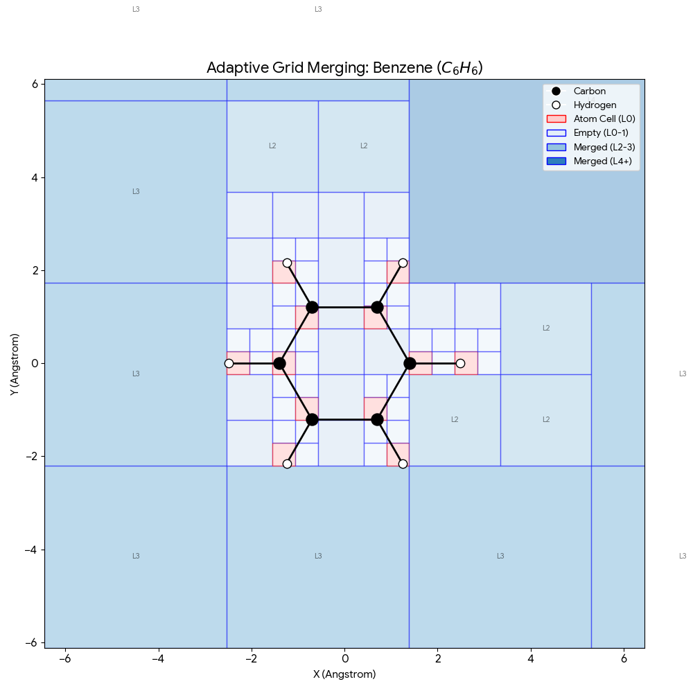
Visualizing Adaptive Grid Merging:

The adaptive grid process compresses empty space around molecules while maintaining high resolution near atoms:
- Red Cells (Level 0): The smallest squares ($0.49$Å) containing atoms. These are kept at highest resolution because electron density changes rapidly here.
- Light Blue Cells (Level 0/1): Small empty regions close to atoms.
- Darker Blue Cells (Level 2/3): Large blocks of empty space further away.
If we used a naive uniform grid, we would have to process thousands of empty “Level 0” cells containing almost zero information. By merging them into larger blocks (the dark blue squares), the model covers the same volume with significantly fewer input tokens, reducing the number of tokens by roughly 10x compared to a dense grid.

The benzene example above demonstrates how this scales to larger molecules. The characteristic hexagonal ring of 6 carbon atoms (black) and 6 hydrogen atoms (white) occupies a small fraction of the total grid. The dark blue corners (L3, L4) represent massive merged blocks of empty space, allowing the model to focus 90% of its computational power on the red “active” zones where chemistry actually happens.
Paper Information
Citation: Lu, S., Ji, X., Zhang, B., Yao, L., Liu, S., Gao, Z., Zhang, L., & Ke, G. (2025). Beyond Atoms: Enhancing Molecular Pretrained Representations with 3D Space Modeling. Proceedings of the 42nd International Conference on Machine Learning (ICML). https://proceedings.mlr.press/v267/lu25e.html
Publication: ICML 2025
@inproceedings{lu2025beyond,
  title={Beyond Atoms: Enhancing Molecular Pretrained Representations with 3D Space Modeling},
  author={Lu, Shuqi and Ji, Xiaohong and Zhang, Bohang and Yao, Lin and Liu, Siyuan and Gao, Zhifeng and Zhang, Linfeng and Ke, Guolin},
  booktitle={Proceedings of the 42nd International Conference on Machine Learning},
  year={2025}
}
Additional Resources: