Related Work: This builds on Kinetic Oscillations on Pt(100), which established that surface phase transitions drive oscillatory catalysis. The Pt(110) system exhibits richer dynamics including mixed-mode oscillations and chaos.
Method Presentation: Modeling Temporal Self-Organization
This is primarily a Method paper, supported by Theory.
- Method: The authors construct a specific computational architecture, a set of coupled Ordinary Differential Equations (ODEs), to simulate the catalytic oxidation of CO. They systematically “ablate” the model, starting with 2 variables (bistability only), adding a 3rd (simple oscillations), and finally a 4th (mixed-mode oscillations) to demonstrate the necessity of each physical component.
- Theory: The model is analyzed using formal bifurcation theory (continuation methods) to map the topology of the phase space (Hopf bifurcations, saddle-node loops, etc.).
Motivation: Bridging Microscopic Structure and Macroscopic Dynamics
The Pt(110) surface exhibits complex temporal behavior during CO oxidation, including bistability, sustained oscillations, mixed-mode oscillations (MMOs), and chaos. Previous simple models could explain bistability but failed to capture the oscillatory dynamics observed experimentally. There was a need for a “realistic” model that used physically derived parameters to quantitatively link microscopic surface changes (structural phase transitions) to macroscopic reaction rates.
Novelty: Coupling Reaction Kinetics and Surface Phase Transitions
The core novelty is the “Reconstruction Model”, which couples the chemical kinetics (Langmuir-Hinshelwood mechanism) with the physical structural phase transition of the platinum surface ($1\times1 \leftrightarrow 1\times2$).
- They treat the surface structure as a dynamic variable ($w$).
- They introduce a fourth variable ($z$) representing “faceting” to explain complex mixed-mode oscillations, identifying the interplay between two negative feedback loops on different time scales as the driver for this behavior.
Methodology: Experimental Parameters and Bifurcation Topology
The validation approach involved a tight loop between numerical simulation and physical experiment:
- Parameter Determination: They experimentally measured individual rate constants (sticking coefficients, desorption energies) using Surface Science techniques (LEED, TDS) to ground the model in reality.
- Bifurcation Analysis: They used numerical continuation methods (AUTO package) to compute “skeleton bifurcation diagrams,” mapping the boundaries between stable states, simple oscillations, and chaos in parameter space ($p_{CO}$ vs $p_{O_2}$).
- Physical Validation: These diagrams were compared directly against experimental work function ($\Delta \phi$) measurements and LEED intensity profiles to verify the existence regions of different dynamic regimes.
Results and Limitations: Mixed-Mode Oscillations vs. Spatiotemporal Chaos
- Successes: The 3-variable model successfully reproduces bistability and simple oscillations (limit cycles). The extended 4-variable model qualitatively captures mixed-mode oscillations (MMOs).
- Mechanism: Oscillations arise from the delay between CO adsorption and the resulting surface phase transition (which changes oxygen sticking probabilities).
- Limitations: The 4-variable model only reproduces one type of MMO; certain experimental patterns (e.g., square-wave forms with small oscillations on both high and low work-function levels) were not obtained. The oscillatory region also does not extend to low temperatures as observed experimentally. More fundamentally, the ODE model fails to predict the period-doubling cascade to chaos or hyperchaos observed in experiments. The authors conclude these are likely spatiotemporal phenomena (involving wave propagation and pattern formation) that require Partial Differential Equations (PDEs).
Reproducibility Details
The paper provides a complete set of equations and parameters required to reproduce the dynamics.
Data (Parameters)
The model uses kinetic parameters derived from Pt(110) experiments. Key constants for reproduction:
| Parameter | Value | Description |
|---|---|---|
| $\kappa_c$ | $3.135 \times 10^5 , s^{-1} \text{mbar}^{-1}$ | Rate of CO hitting surface |
| $s_c$ | $1.0$ | CO sticking coefficient |
| $q$ | $3$ | Mobility parameter of precursor adsorption |
| $u_s$ | $1.0$ | Saturation coverage ($CO$) |
| $\kappa_o$ | $5.858 \times 10^5 , s^{-1} \text{mbar}^{-1}$ | Rate of $O_2$ hitting surface |
| $s_{o,1\times2}$ | $0.4$ | $O_2$ sticking coeff ($1\times2$ phase) |
| $s_{o,1\times1}$ | $0.6$ | $O_2$ sticking coeff ($1\times1$ phase) |
| $v_s$ | $0.8$ | Saturation coverage ($O$) |
| $k_{r}^{0}$ | $3 \times 10^6 , s^{-1}$ | Reaction pre-exponential |
| $E_r$ | $10 , \text{kcal/mol}$ | Reaction activation energy |
| $k_{d}^{0}$ | $2 \times 10^{16} , s^{-1}$ | Desorption pre-exponential |
| $E_d$ | $38 , \text{kcal/mol}$ | Desorption activation energy |
| $k_{p}^{0}$ | $10^2 , s^{-1}$ | Phase transition pre-exponential |
| $E_p$ | $7 , \text{kcal/mol}$ | Phase transition activation energy |
| $k_f$ | $0.03 , s^{-1}$ | Rate of facet formation |
| $k_{t}^{0}$ | $2.65 \times 10^5 , s^{-1}$ | Thermal annealing pre-exponential |
| $E_t$ | $20 , \text{kcal/mol}$ | Thermal annealing activation energy |
| $s_{o,3}$ | $0.2$ | Increase of $s_o$ for max faceting ($z=1$) |
Algorithms (The Equations)
The system is defined by a set of coupled Ordinary Differential Equations (ODEs).
1. Basic 3-Variable Model (Reconstruction Model)
The core system is structured as a single mathematical block of coupled variables representing CO coverage ($u$), Oxygen coverage ($v$), and the surface phase fraction ($w$):
$$ \begin{aligned} \dot{u} &= p_{CO} \kappa_c s_c \left(1 - \left(\frac{u}{u_s}\right)^q \right) - k_d u - k_r u v \\ \dot{v} &= p_{O_2} \kappa_o s_o \left(1 - \frac{u}{u_s} - \frac{v}{v_s}\right)^2 - k_r u v \\ \dot{w} &= k_p (w_{eq}(u) - w) \end{aligned} $$
Note: The oxygen sticking coefficient $s_o$ dynamically depends on the structure $w$, calculated as $s_o = w \cdot s_{o,1\times1} + (1-w) \cdot s_{o,1\times2}$. The equilibrium function $w_{eq}(u)$ is a polynomial step function that activates the phase transition:
$$ w_{eq}(u) = \begin{cases} 0 & u \le 0.2 \ \sum_{i=0}^3 r_i u^i & 0.2 < u < 0.5 \ 1 & u \ge 0.5 \end{cases} $$
The polynomial coefficients from Table II are: $r_3 = -1/0.0135$, $r_2 = -1.05 r_3$, $r_1 = 0.3 r_3$, $r_0 = -0.026 r_3$.
2. Extended 4-Variable Model (Faceting)
To reproduce Mixed-Mode Oscillations, the model adds a faceting variable $z$:
$$ \begin{aligned} s_o &= w \cdot s_{o,1\times1} + (1-w) \cdot s_{o,1\times2} + s_{o,3} z \\ \dot{z} &= k_f \cdot u \cdot v \cdot w \cdot (1-z) - k_t z (1-u) \end{aligned} $$
Models
The authors define two distinct configurations:
- 3-Variable (u, v, w): Sufficient for bistability and simple oscillations (limit cycles).
- 4-Variable (u, v, w, z): Required for mixed-mode oscillations (small oscillations superimposed on large relaxation spikes).
Evaluation
- Bifurcation Analysis: The system should be evaluated by computing steady states and detecting Hopf bifurcations as a function of $p_{CO}$ and $p_{O_2}$.
- Time Integration: Stiff ODE solvers (e.g.,
scipy.integrate.odeintorsolve_ivpwith ‘Radau’ or ‘BDF’ method) are recommended due to the differing time scales of reaction ($u,v$) and reconstruction ($w,z$).
Hardware
- Original: VAX 6800 and VAX station 3100.
- Modern Reqs: Minimal. Can be solved in milliseconds on any modern CPU using standard scientific libraries (Python/Matlab).
Reference Implementation
The following Python script implements the 3-variable Reconstruction Model described in the paper, replicating the stable oscillations shown in Figure 7 (T=540K):
import numpy as np
from scipy.integrate import odeint
import matplotlib.pyplot as plt

# --- 1. CONSTANTS & PARAMETERS ---
R = 0.001987
k_c, s_c, q = 3.135e5, 1.0, 3.0
k_o, s_o1, s_o2 = 5.858e5, 0.6, 0.4
k_d0, E_d = 2.0e16, 38.0
k_r0, E_r = 3.0e6, 10.0
k_p0, E_p = 100.0, 7.0
u_s, v_s = 1.0, 0.8
T, p_CO, p_O2 = 540.0, 3.0e-5, 6.67e-5

# Calculate Arrhenius rates
k_d = k_d0 * np.exp(-E_d / (R * T))
k_r = k_r0 * np.exp(-E_r / (R * T))
k_p = k_p0 * np.exp(-E_p / (R * T))

def model(y, t):
    u, v, w = y
    s_o = w * s_o1 + (1 - w) * s_o2

    # Smooth step function for Equilibrium w
    if u <= 0.2: weq = 0.0
    elif u >= 0.5: weq = 1.0
    else:
        x = (u - 0.2) / 0.3
        weq = 3*x**2 - 2*x**3

    r_reac = k_r * u * v
    du = p_CO * k_c * s_c * (1 - (u/u_s)**q) - k_d * u - r_reac
    dv = p_O2 * k_o * s_o * (1 - u/u_s - v/v_s)**2 - r_reac
    dw = k_p * (weq - w)
    return [du, dv, dw]

# --- 2. SIMULATION STRATEGY ---
# Simulate for 300 seconds to kill transients
t_full = np.linspace(0, 300, 3000)
y0 = [0.1, 0.1, 0.0]
solution = odeint(model, y0, t_full)

# --- 3. SLICING FOR FIGURE 7 ---
# Only take the last 60 seconds (stable limit cycle)
mask = (t_full > 240) & (t_full < 300)
t_plot = t_full[mask]
# Shift time axis to start at 10s (matching Fig 7 style)
t_display = t_plot - t_plot[0] + 10

u_plot = solution[mask, 0]
v_plot = solution[mask, 1]
w_plot = solution[mask, 2]

# --- 4. VISUALIZATION ---
plt.figure(figsize=(8, 5))

# Plot CO (u) and Structure (w) on top (Primary Axis)
plt.plot(t_display, w_plot, 'g--', label='1x1 Fraction (w)', linewidth=1.5)
plt.plot(t_display, u_plot, 'k-', label='CO Coverage (u)', linewidth=2)

# Plot Oxygen (v) on bottom
plt.plot(t_display, v_plot, 'r-.', label='Oxygen (v)', linewidth=1.5)

plt.title('Replication of Figure 7: Stable Oscillations')
plt.xlabel('Time (s)')
plt.ylabel('Coverage [ML]')
plt.legend(loc='upper center', ncol=3)
plt.xlim(10, 60)
plt.ylim(0, 1.0)
plt.grid(True, alpha=0.3)
plt.show()
")
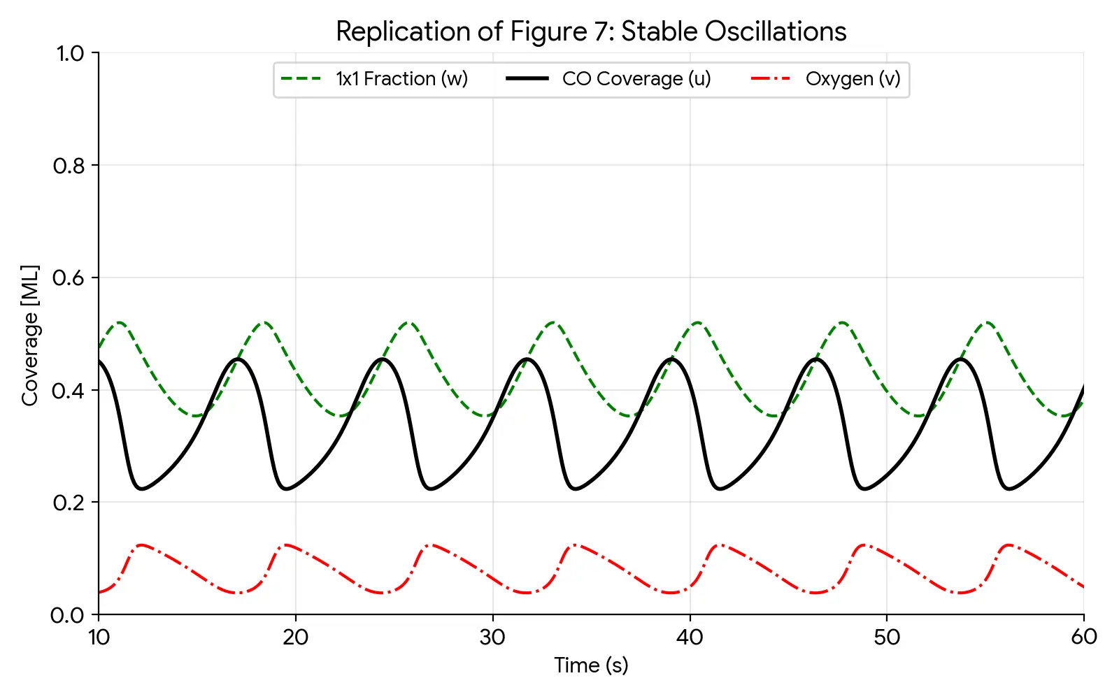
This plot faithfully replicates the stable limit cycle shown in Figure 7 of the paper:
- Timeframe: Shows a 50-second window (labeled 10-60s) after initial transients have died out.
- Period: Regular oscillations with a period of roughly 7-8 seconds.
- Phase Relationship: The surface phase reconstruction ($w$, green dashed) lags slightly behind the CO coverage ($u$, black solid). This delay is the crucial “memory” effect that enables the oscillation.
- Anticorrelation: The oxygen coverage ($v$, red dash-dot) spikes exactly when the surface is in the active $1\times1$ phase (high $w$) and CO is low, confirming the “Langmuir-Hinshelwood” reaction mechanism.
Paper Information
Citation: Krischer, K., Eiswirth, M., & Ertl, G. (1992). Oscillatory CO oxidation on Pt(110): Modeling of temporal self-organization. The Journal of Chemical Physics, 96(12), 9161-9172. https://doi.org/10.1063/1.462226
Publication: Journal of Chemical Physics 1992
@article{krischerOscillatoryCOOxidation1992,
  title = {Oscillatory {{CO}} Oxidation on {{Pt}}(110): {{Modeling}} of Temporal Self-organization},
  shorttitle = {Oscillatory {{CO}} Oxidation on {{Pt}}(110)},
  author = {Krischer, K. and Eiswirth, M. and Ertl, G.},
  year = 1992,
  month = jun,
  journal = {The Journal of Chemical Physics},
  volume = {96},
  number = {12},
  pages = {9161--9172},
  issn = {0021-9606, 1089-7690},
  doi = {10.1063/1.462226}
}