Methodological Validation and Physical Discovery
This is primarily a Methodological Paper ($\Psi_{\text{Method}}$), with a significant secondary component of Discovery ($\Psi_{\text{Discovery}}$).
It focuses on validating a specific algorithm (the “Evans method”) for Non-Equilibrium Molecular Dynamics (NEMD) by comparing its results against experimental benchmarks. However, it also uncovers physical anomalies, specifically “long-time tails” in the heat flux autocorrelation function that deviate significantly from theoretical predictions, marking a discovery about the physics of the Lennard-Jones fluid itself.
Flow Gradients and Boundary Limitations
The primary motivation is to overcome the limitations of simulating heat flow using physical boundaries (e.g., walls at different temperatures), which causes severe interpretive difficulties due to density and temperature gradients.
The “Evans method” uses a fictitious external field to induce heat flow in a periodic, homogeneous system. This paper serves to:
- Validate this method across a wide range of state points (temperatures and densities) beyond the triple point.
- Investigate the system’s behavior near the critical point, where transport properties are known to be anomalous.
Core Innovations of the Evans Algorithm
The core contribution is the rigorous stress-testing of the homogeneous heat flow algorithm (Evans method) combined with a Gaussian thermostat.
Specific novel insights include:
- Linearity Validation: Establishing that, away from phase boundaries, the effective thermal conductivity is a monotonic, virtually linear function of the external field, justifying the extrapolation to zero field.
- Critical Anomaly Detection: Finding that near the critical point, conductivity becomes a non-monotonic function of the field, challenging standard simulation approaches in this regime.
- Tail Amplitude Discovery: Demonstrating that the “long-time tails” of the heat flux autocorrelation function have amplitudes roughly 6 times larger than those predicted by mode-coupling theory.
NEMD Simulation Setup
The author performed Non-Equilibrium Molecular Dynamics (NEMD) simulations using the Lennard-Jones potential.
- System: Mostly $N=108$ particles, with some checks using $N=256$ to test size dependence.
- Thermostat: A Gaussian thermostat was used to keep the kinetic energy (temperature) constant.
- State Points:
- Critical Isotherm: $T=1.35$, varying density.
- Supercritical Isotherm: $T=2.0$.
- Freezing Line: Two points ($T=2.74, \rho=1.113$ and $T=2.0, \rho=1.04$).
- Validation: Results were compared against experimental data for Argon (using standard LJ parameters).
- Ablation:
- Field Strength ($F$): Varied to check for linearity/non-linearity.
- System Size ($N$): Comparison between 108 and 256 particles to rule out finite-size artifacts.
Linearity Regimes and Long-Time Tail Anomalies
- Agreement with Experiment: The Evans method yields thermal conductivities in broad agreement with experimental Argon data for most state points.
- Linearity: Away from the critical point, conductivity is a virtually linear function of the field strength $F$, allowing for accurate zero-field extrapolation.
- Critical Region Failure: Near the critical point ($T=1.35, \rho=0.4$), the method struggles; the conductivity is non-monotonic with respect to $F$, and the zero-field extrapolation underestimates the experimental value by ~11%.
- Long-Time Tails: The decay of the heat flux autocorrelation function follows a $t^{-3/2}$ tail (consistent with mode-coupling theory), but the amplitude is ~6x larger than predicted.
- Phase Hysteresis: In high-density regions near the freezing line, the system exhibits hysteresis and bi-stability between solid and liquid phases depending on the field strength.
Reproducibility Details
Data
The simulation relies on the Lennard-Jones (LJ) potential to model Argon. No external training data is used; the “data” consists of the physical constants defining the system.
| Parameter | Value/Description | Notes |
|---|---|---|
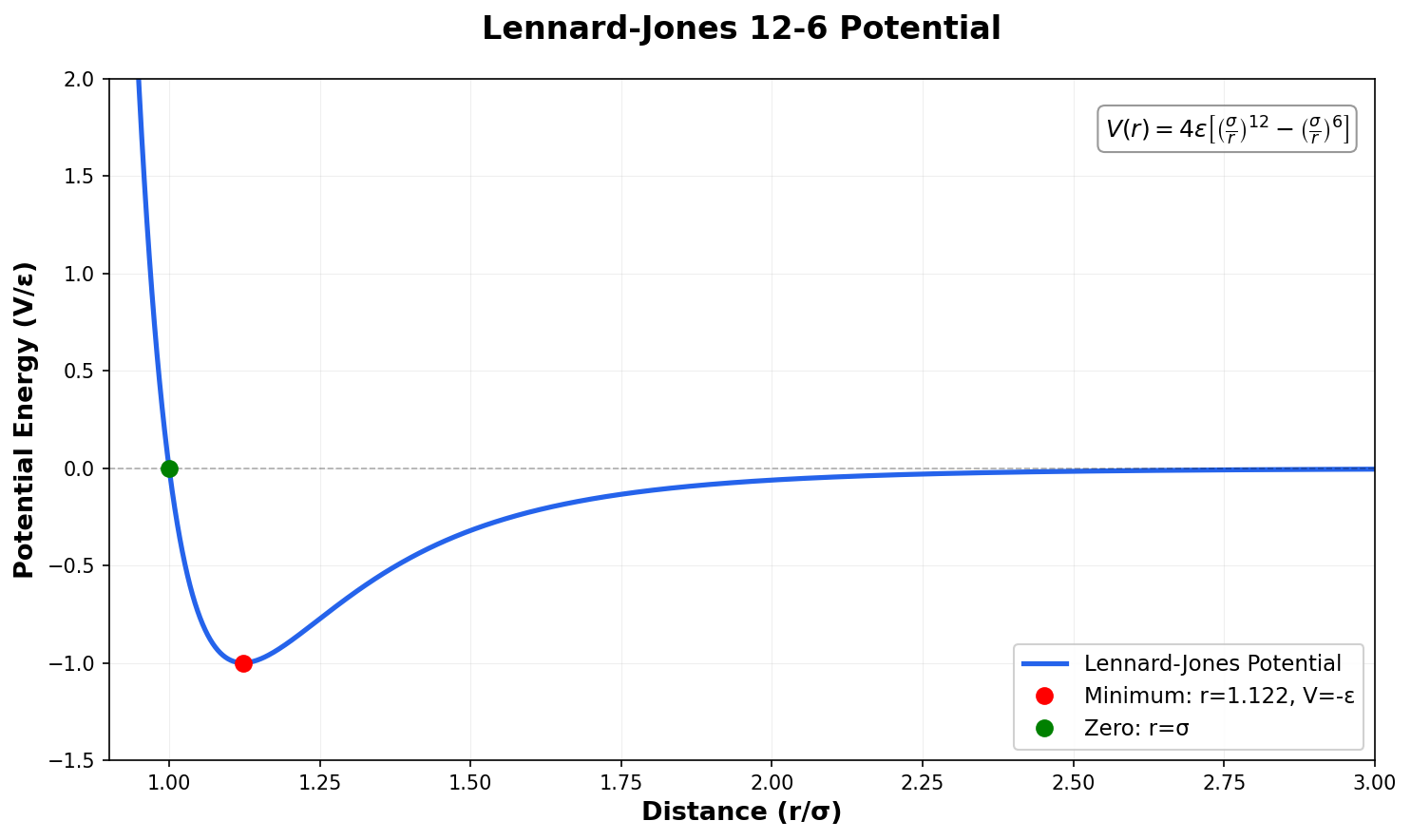
| Potential | $\Phi(q)=4(q^{-12}-q^{-6})$ | Standard LJ 12-6 potential |
| Cutoff | $r_c = 2.5$ | Truncated at 2.5 distance units |
| Comparison | Argon Experimental Data | Sourced from NBS recommended values |
Algorithms
The core algorithm is the Evans Homogeneous Heat Flow method. To reproduce this, one must implement the specific Equations of Motion (EOM) derived from linear response theory.
Equations of Motion:
The trajectories are generated by: $$ \begin{aligned} \dot{q}_i &= \frac{p_i}{m} \\ \dot{p}_i &= F_i^{\text{inter}} + (E_i - \bar{E})F(t) - \sum_{j} F_{ij} q_{ij} \cdot F(t) + \frac{1}{2N} \sum_{j,k} F_{jk} q_{jk} \cdot F(t) - \alpha p_i \end{aligned} $$
Where:
- $F(t)$ is the fictitious external field driving heat flow.
- $E_i$ is the instantaneous energy of particle $i$.
- $\alpha$ is the Gaussian Thermostat multiplier (calculated at every step to strictly conserve kinetic energy/Temperature): $$\alpha = \frac{\sum_i [\dots]_{\text{force terms}} \cdot p_i}{\sum_i p_i \cdot p_i}$$
Conductivity Calculation:
The zero-frequency limit is extrapolated as: $$ \lambda = \lim_{F \to 0} \frac{J_Q}{FT} $$
The frequency-dependent conductivity relies on the heat-flux autocorrelation: $$ \lambda(\omega) = \frac{V}{3k_B T^2} \int_0^\infty dt , e^{i\omega t} \langle J_Q(t) \cdot J_Q(0) \rangle $$
Models
The “model” here is the physical simulation setup.
- Particle Count: $N = 108$ (primary), $N = 256$ (validation).
- Boundary Conditions: Periodic Boundary Conditions (PBC).
- Thermostat: Gaussian Isokinetic (Temperature is a constant of motion).
Evaluation
The primary metric is the Thermal Conductivity ($\lambda$).
| Metric | Definition | Baseline | Result |
|---|---|---|---|
| Thermal Conductivity | Ratio of heat flux $J_Q$ to field $F$ (extrapolated to $F=0$) | Experimental Argon (NBS Data) | Good agreement away from critical point |
| Tail Amplitude | Coefficient of the $\omega^{1/2}$ term in frequency-dependent conductivity | Mode-Coupling Theory ($\approx 0.05$) | Simulation value $\approx 0.3$ (6x larger) |
Hardware
- Requirements: While 1986 hardware is obsolete, reproducing this requires a standard MD code capable of non-conservative forces (NEMD).
- Compute Cost: Low by modern standards. 108 particles for $\sim 10^5$ to $10^6$ steps is trivial on modern CPUs.
Paper Information
Citation: Evans, D. J. (1986). Thermal conductivity of the Lennard-Jones fluid. Physical Review A, 34(2), 1449-1453. https://doi.org/10.1103/PhysRevA.34.1449
Publication: Physical Review A, 1986
@article{PhysRevA.34.1449,
  title = {Thermal conductivity of the Lennard-Jones fluid},
  author = {Evans, Denis J.},
  journal = {Phys. Rev. A},
  volume = {34},
  issue = {2},
  pages = {1449--1453},
  numpages = {0},
  year = {1986},
  month = {Aug},
  publisher = {American Physical Society},
  doi = {10.1103/PhysRevA.34.1449},
  url = {https://link.aps.org/doi/10.1103/PhysRevA.34.1449}
}