Overview
The Müller-Brown potential is a primary benchmark system in computational chemistry: a two-dimensional analytical surface used to evaluate optimization algorithms. Introduced by Klaus Müller and Leo D. Brown in 1979 as a test system for their constrained simplex optimization algorithm, this potential energy function captures the essential topology of chemical reaction landscapes while preserving computational efficiency.
Origin: Müller, K., & Brown, L. D. (1979). Location of saddle points and minimum energy paths by a constrained simplex optimization procedure. Theoretica Chimica Acta, 53, 75-93. The potential is introduced in footnote 7 (p. 79) as a two-parametric model surface for testing the constrained simplex procedures.
Mathematical Definition
The Müller-Brown potential combines four two-dimensional Gaussian functions:
$$V(x,y) = \sum_{k=1}^{4} A_k \exp\left[a_k(x-x_k^0)^2 + b_k(x-x_k^0)(y-y_k^0) + c_k(y-y_k^0)^2\right]$$
Each Gaussian contributes a different “bump” or “well” to the landscape. The parameters control amplitude ($A_k$), width, orientation, and center position.
Standard Parameters
The canonical parameter values that define the Müller-Brown surface are:
| k | $A_k$ | $a_k$ | $b_k$ | $c_k$ | $x_k^0$ | $y_k^0$ |
|---|---|---|---|---|---|---|
| 1 | -200 | -1 | 0 | -10 | 1 | 0 |
| 2 | -100 | -1 | 0 | -10 | 0 | 0.5 |
| 3 | -170 | -6.5 | 11 | -6.5 | -0.5 | 1.5 |
| 4 | 15 | 0.7 | 0.6 | 0.7 | -1 | 1 |
The first three terms have negative amplitudes (creating energy wells), while the fourth has a positive amplitude (creating a barrier). The cross-term $b_k$ in the third Gaussian creates the tilted orientation that gives the surface its characteristic curved pathways.
Analytical Gradients (Forces)
To optimize paths or simulate molecular dynamics across this surface, calculating the spatial derivatives (negative forces) is structurally simple. Defining $G_k(x,y)$ as the inner argument of the exponent, the partial derivatives with respect to $x$ and $y$ are:
$$ \frac{\partial V}{\partial x} = \sum_{k=1}^4 A_k \exp[G_k(x,y)] \cdot \left[ 2a_k(x-x_k^0) + b_k(y-y_k^0) \right] $$
$$ \frac{\partial V}{\partial y} = \sum_{k=1}^4 A_k \exp[G_k(x,y)] \cdot \left[ b_k(x-x_k^0) + 2c_k(y-y_k^0) \right] $$
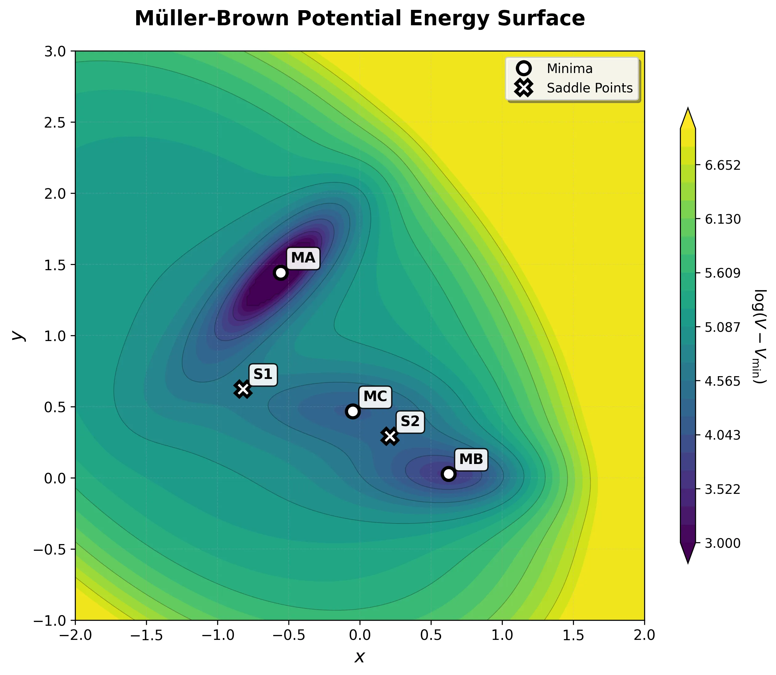
Energy Landscape
This simple formula creates a surprisingly rich topography with exactly the features needed to challenge optimization algorithms:
| Stationary Point | Coordinates | Energy | Type |
|---|---|---|---|
| MA (Reactant) | (-0.558, 1.442) | -146.70 | Deep minimum |
| MC (Intermediate) | (-0.050, 0.467) | -80.77 | Shallow minimum |
| MB (Product) | (0.623, 0.028) | -108.17 | Medium minimum |
| S1 | (-0.822, 0.624) | -40.67 | First saddle point |
| S2 | (0.212, 0.293) | -72.25 | Second saddle point |
All values from Table 1 of Müller & Brown (1979).
 and two saddle points")
Key Challenge: Curved Reaction Pathways
The path from the deep reactant minimum (MA) to the product minimum (MB) follows a curved two-step pathway:
- MA → S1 → MC: First transition over a lower barrier into an intermediate basin
- MC → S2 → MB: Second transition over a slightly higher barrier to the product
This curved pathway breaks linear interpolation methods. Algorithms that draw a straight line from reactant to product miss both the intermediate minimum and the correct transition states, climbing over much higher energy regions instead.
Why It Works as a Benchmark
The Müller-Brown potential has served as a computational chemistry benchmark for over four decades because of four key characteristics:
Low dimensionality: As a 2D surface, it permits complete visualization of the landscape, clearly revealing why specific algorithms succeed or fail.
Analytical form: Energy and gradient calculations cost virtually nothing, enabling exhaustive testing impossible with quantum mechanical surfaces.
Non-trivial topology: The curved minimum energy path and shallow intermediate minimum challenge sophisticated methods while remaining manageable.
Known ground truth: All minima and saddle points are precisely known, providing unambiguous success metrics.
Contrast with Other Benchmarks
The Müller-Brown potential provides distinct evaluation metrics compared to other classic potentials. The Lennard-Jones potential serves as the standard benchmark for equilibrium properties due to its single energy minimum. In parallel, Müller-Brown explicitly models reactive landscapes. Its multiple minima and connecting barriers create an evaluation environment for algorithms designed to discover transition states and reaction paths.
Historical Applications
The potential has evolved with the field’s changing focus:
1980s-1990s: Testing path-finding methods like Nudged Elastic Band (NEB), which creates discrete representations of reaction pathways and optimizes them to find minimum energy paths.
2000s-2010s: Validating Transition Path Sampling (TPS) methods that harvest statistical ensembles of reactive trajectories.
2020s: Benchmarking machine learning models and generative approaches that learn to sample transition paths or approximate potential energy surfaces.
Modern Applications in Machine Learning
The rise of machine learning has given the Müller-Brown potential renewed purpose. Modern Machine Learning Interatomic Potentials (MLIPs) aim to bridge the gap between quantum mechanical accuracy and classical force field efficiency by training flexible models on expensive quantum chemistry data.
The Müller-Brown potential provides an ideal benchmarking solution: an exactly known potential energy surface that can generate unlimited, noise-free training data. This enables researchers to ask fundamental questions:
- How well does a given architecture learn complex, curved surfaces?
- How many training points are needed for acceptable accuracy?
- How does the model behave when extrapolating beyond training data?
- Can it correctly identify minima and saddle points?
The potential serves as a consistent benchmark for measuring the learning capacity of AI models.
Extensions and Variants
Higher-Dimensional Extensions
The canonical Müller-Brown potential can be extended beyond two dimensions to create more challenging test cases:
Harmonic constraints: Add quadratic wells in orthogonal dimensions while preserving the complex 2D landscape:
$$V_{5D}(x_1, x_2, x_3, x_4, x_5) = V(x_1, x_3) + \kappa(x_2^2 + x_4^2 + x_5^2)$$
Collective variables (CVs): Collective variables are low-dimensional coordinates that capture the most important degrees of freedom in a high-dimensional system. By defining CVs that mix multiple dimensions, the original surface can be embedded in higher-dimensional spaces. For instance, the active 2D coordinates $x$ and $y$ can be projected as linear combinations of $N$ arbitrary degrees of freedom ($q_i$):
$$ x = \sum_{i=1}^N w_{x,i} q_i \quad \text{and} \quad y = \sum_{i=1}^N w_{y,i} q_i $$
This constructs a complex, high-dimensional problem where an algorithm must learn to isolate the relevant active subspace (the CVs) before it can effectively optimize the topology.
These extensions enable systematic testing of algorithm scaling with dimensionality while maintaining known ground truth in the active subspace.
Limitations
Despite its utility, the Müller-Brown potential has fundamental limitations as a proxy for physical systems:
- Lack of Realistic Scaling: As a purely mathematical 2D/analytical model, it cannot directly simulate the complexities of high-dimensional scaling found in many-body atomic systems.
- No Entropic Effects: In real chemical systems, entropic contributions heavily influence the free-energy landscape. The Müller-Brown potential maps energy precisely but lacks the thermal/entropic complexity of solvent or macromolecular environments.
- Trivial Topology Contrasts: While non-trivial compared to single wells, its global topology remains simpler than proper ab initio potential energy surfaces, missing features like complex bifurcations, multi-state crossings, or non-adiabatic couplings.
Implementation Considerations
Modern implementations typically focus on:
- Vectorized calculations for batch processing
- Analytical derivatives for gradient-based methods
- JIT compilation for performance optimization
- Automatic differentiation compatibility for machine learning frameworks
The analytical nature of the potential makes it ideal for testing both classical optimization methods and modern machine learning approaches.
Resources and Visualizations
- Interactive Müller-Brown Potential Energy Surface - Local visualization tool
- Müller-Brown Potential Visualization (Wolfram) - External Wolfram demonstration
- Implementing the Müller-Brown Potential in PyTorch - Detailed implementation guide with performance analysis
Related Systems
The Müller-Brown potential belongs to a family of analytical benchmark systems used in computational chemistry. Other notable examples include:
- Lennard-Jones potential: Single-minimum benchmark for equilibrium properties
- Double-well potentials: Simple models for bistable systems
- Eckart barrier: One-dimensional tunneling benchmark
- Wolfe-Quapp potential: Higher-dimensional extension with valley-ridge inflection points
Conclusion
The Müller-Brown potential demonstrates how a well-designed benchmark can evolve with a field. Originating from 1970s computational constraints to test algorithms when quantum chemistry calculations were expensive, its topology causes naive linear-interpolation approaches to fail while maintaining instantaneous computational execution. Because of this, it remains a heavily analyzed benchmark system today.
It serves specific purposes in the machine learning era by providing a controlled environment for developing methods targeted at complex realistic molecular systems. Its evolution from a practical surrogate model to a machine learning benchmark demonstrates the continued relevance of foundational analytical test cases in computational science.