What is a word embedding?
A word embedding is a real-valued vector representation of a word: $$ \text{word} \rightarrow \mathbb{R}^n $$ for some $n$, where $n$ is the integer dimensionality of the word embedding space.
Ideally, words with similar meaning will have vector representations that are close together in the embedding space. This allows us to use mathematical operations on the vectors to capture relationships between words.
When constructing a word embedding space, typically the goal is to capture some sort of relationship in that space, be it meaning, context, or syntax. By encoding word embeddings in a densely populated space, we can represent words numerically in a way that captures them in vectors that have tens or hundreds of dimensions instead of millions (like one-hot encoded vectors).
A foundational idea behind word embeddings is Zellig Harris’ “distributional hypothesis”, the idea that words that are used and occur in the same contexts tend to have similar meanings. This is the basis of distributional semantics.

Distributional Semantics: An illustrative example of words embedded in a three-dimensional space, loosely organized by meaning (source, license)
One beauty is that word embeddings that are created with different algorithms or data can capture different aspects of the distributional hypothesis. The end result are word embeddings that help us on different down-stream tasks. In this post, we’ll discuss some of the different ways one can numerically represent words and how they are used in natural language processing (NLP).
Why do we use word embeddings in NLP?
Words are not inherently understandable to computers in their raw form. To bridge this gap, we encode words into numeric formats, enabling the application of mathematical operations and matrix manipulations. This numeric transformation unlocks their potential within the realm of machine learning, particularly in deep learning.
In deep learning, numerical representations of words allow us to leverage various architectures for processing language. Convolutional Neural Networks (CNNs), for instance, have been adapted to handle Natural Language Processing (NLP) tasks by utilizing word embeddings, achieving state-of-the-art results in several domains.
An even more promising development is the ability to pre-train word embeddings that are versatile across multiple tasks. This article will explore such embeddings in depth. The advantage here is significant: rather than crafting a unique set of embeddings for each task and dataset, we can develop universal representations that serve a broad spectrum of applications. This approach simplifies the process, making powerful NLP tools more accessible and efficient.
Specific examples of word embeddings in NLP
One-Hot Encoding (Count Vectorizing)
One of the most basic ways we can numerically represent words is through the one-hot encoding method (also sometimes called count vectorizing).
The idea is simple. Create a vector that has as many dimensions as your corpora has unique words. Each unique word has a unique dimension and will be represented by a 1 in that dimension and 0 in all other dimensions.
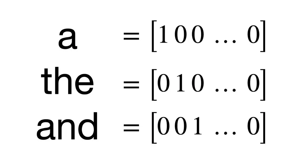
One-Hot Encoding: A visual representation of one-hot encoding for the words ‘a’, ’the’, and ‘and’
The result of this? Really huge and sparse vectors that capture absolutely no relational information. It could be useful if you have no other option. But we do have other options, if we need that semantic relationship information.
TF-IDF Transform
TF-IDF vectors are related to one-hot encoded vectors. However, instead of just featuring a count, they feature numerical representations where words aren’t just there or not there. Instead, words are represented by their term frequency (TF) multiplied by their inverse document frequency (IDF).
In simpler terms, words that occur a lot but everywhere should be given very
little weighting or significance. We can think of this as words like the or
and in the English language. They don’t provide a large amount of value.
However, if a word appears very little or appears frequently, but only in one or two places, then these are probably more important words and should be weighted as such.
Again, this suffers from the downside of very high dimensional representations that don’t necessarily capture semantic relationships. But they do contain more useful information, particularly in exposing document and broader topic relationships.
Co-Occurrence Matrix
A co-occurrence matrix is exactly what it sounds like: a giant matrix that is as long and as wide as the vocabulary size. If words occur together, they are marked with a positive entry. Otherwise, they have a 0. It boils down to a numeric representation that simply asks “Do words occur together? If yes, then count this.”
And what can we already see becoming a big problem? Super large representation! If we thought that one-hot encoding was high dimensional, then co-occurrence is high dimensional squared. That’s a lot of data to store in memory.

Co-Occurrence Matrix: A visual representation of a co-occurrence matrix for a range of three words. The source sentence was: ‘The dawn is the appearance of light - usually golden, pink or purple - before sunrise.’
Neural Probabilistic Model
Now, we can start to get into some neural networks. A neural probabilistic model learns an embedding by achieving some task like modeling or classification and is what the rest of the widely used word embeddings are based on.
Typically, you clean your text and create one-hot encoded vectors. Then, you define your representation size (300 dimensional might be good). From there, we initialize the embedding to random values. It’s the entry point into the network, and back-propagation is utilized to modify the embedding based on whatever goal task we have.
This typically takes a lot of data and can be very slow. The trade-off here is that it learns an embedding that is good for the text data that the network was trained on as well as the NLP task that was jointly learned during training.

Neural Probabilistic Model: A visual representation of a neural probabilistic model
word2vec
Word2Vec is a better successor to the neural probabilistic model. We still use a statistical computation method to learn from a text corpus, however, its method of training is more efficient than just simple embedding training. It is more or less the standard method for training embeddings the days.
It is also the first method that demonstrated classic vector arithmetic to create analogies:

Word2Vec: A visual representation of word2vec (source, license)
There are two major learning approaches.
Continuous Bag-of-Words (CBOW)
This method learns an embedding by predicting the current words based on the context. The context is determined by the surrounding words.
Continuous Skip-Gram
This method learns an embedding by predicting the surrounding words given the context. The context is the current word.
Both of these learning methods use local word usage context (with a defined window of neighboring words). The larger the window is, the more topical similarities that are learned by the embedding. Forcing a smaller window results in more semantic, syntactic, and functional similarities to be learned.
So, what are the benefits? Well, high quality embeddings can be learned pretty efficiently, especially when comparing against neural probabilistic models. That means low space and low time complexity to generate a rich representation. More than that, the larger the dimensionality, the more features we can have in our representation. But still, we can keep the dimensionality a lot lower than some other methods. It also allows us to efficiently generate something like a billion word corpora, but encompass a bunch of generalities and keep the dimensionality small.
GloVe
GloVe is an extension of word2vec, and a much better one at that. There are a set of classical vector models used for natural language processing that are good at capturing global statistics of a corpus, like LSA (matrix factorization). They’re very good at global information, but they don’t capture meanings so well and definitely don’t have the cool analogy features built in.
GloVe’s contribution was the addition of global statistics in the language modeling task to generate the embedding. There is no window feature for local context. Instead, there is a word-context/word co-occurrence matrix that learns statistics across the entire corpora.
The result? A much better embedding being learned than simple word2vec.
FastText
Now, with FastText we enter into the world of really cool recent word embeddings. What FastText did was decide to incorporate sub-word information. It did so by splitting all words into a bag of n-gram characters (typically of size 3-6). It would add these sub-words together to create a whole word as a final feature. The thing that makes this really powerful is it allows FastText to naturally support out-of-vocabulary words!
This is huge because in other approaches, if the system encounters a word that it doesn’t recognize, it just has to set it to the unknown word. With FastText, we can give meaning to words like circumnavigate if we only know the word navigate, because our semantic knowledge of the word navigate can help use at least provide a bit more semantic information to circumnavigate, even if it is not a word our system learned during training.
Beyond that, FastText uses the skip-gram objective with negative sampling. All sub-words are positive examples, and then random samples from a dictionary of words in the corpora are used as negative examples. These are the major things that FastText included in its training.
Another really cool thing is that Facebook, in developing FastText, has published pre-trained FastText vectors in 294 different languages. This is something extremely awesome, in my opinion, because it allows developers to jump into making projects in languages that typically don’t have pre-trained word vectors at a very low cost (since training their own word embeddings takes a lot of computational resources).
If you want to see all the languages that FastText supports, check it out here.
Poincare Embeddings (Hierarchal Representations)
Poincare embeddings are really different and really interesting, and if you are feeling ambitious, you should definitely give the paper a read. They decide to use hyperbolic geometry to capture hierarchal properties of words. By placing their embedding into a hyperbolic space, they can use properties of hyperbolic space to use distance to encode similarity and the norm of vectors to encode hierarchal relationships.
The end result is that less dimensions are needed in order to encode hierarchal information, which they demonstrate by recreating WordNet with very low dimensionality, especially when compared to other word embedding schemes. They highlight how this approach is super useful for data that is extremely hierarchal like WordNet or like a computer network. It will be interesting to see what kind of research, if any, comes out of this stream.
ELMo
ELMo is a personal favorite of mine. They are state-of-the-art contextual word vectors. The representations are generated from a function of the entire sentence to create word-level representations. The embeddings are generated at a character-level, so they can capitalize on sub-word units like FastText and do not suffer from the issue of out-of-vocabulary words.
ELMo is trained as a bi-directional, two layer LSTM language model. An interesting side effect is that its final output is actually a combination of its inner layer outputs. What has been found is that the lowest layer is good for things like POS tagging and other more syntactic and functional tasks, whereas the higher layer is good for things like word-sense disambiguation and other higher-level, more abstract tasks. When we combine these layers, we find that we actually get incredibly high performance on downstream tasks out of the box.
The only questions on my mind? How can we reduce the dimensionality and extend to training on less popular languages like we have for FastText.
Probabilistic FastText
Probabilistic FastText is a paper that came out that tried to better handle the issue of words that have different meanings, but are spelled the same. Take for example the word rock. It can mean:
- Rock music
- A stone
- The action of moving back and forth
How do we know what we are talking about when we encounter this word? Typically, we don’t. When learning an embedding, we just smash all the meanings together and hope for the best. That’s why things like ELMo, which use the entire sentence as a context, tend to perform better when needing to distinguish the different meanings.
That’s also what Probabilistic FastText does really well. Instead of representing words as vectors, words are represented as Gaussian mixture models. Instead of learning a vector, we learn a distribution. This allows us to represent the different meanings of a word as different distributions, which allows us to better capture the different meanings of a word.
Conclusion
Word embeddings are a powerful tool in the NLP toolkit. They allow us to represent words in a way that captures their meaning, context, and syntax. They are used in a variety of NLP tasks and are a foundational concept in the field of NLP. There are many different ways to create word embeddings, and each method has its own strengths and weaknesses. The choice of which method to use depends on the specific task at hand and the data available. In this post, we discussed some of the most popular methods for creating word embeddings and explored their strengths and weaknesses. We hope that this post has given you a better understanding of word embeddings and how they are used in NLP.