Understanding Generative Models
Modern generative AI is dominated by diffusion models and autoregressive transformers. The adversarial training dynamics and objective functions pioneered by Generative Adversarial Networks (GANs) remain critical for stabilizing distributed training and designing robust loss functions today. Before diving into GANs, let’s establish what we’re trying to accomplish with generative models.
The core goal: Create a system that can generate new, realistic data that appears to come from the same distribution as our training data.
Think of having a model that can create images, text, or audio that are difficult to distinguish from human-created content. This is what generative modeling aims to achieve.
The Mathematical Foundation
Generative models aim to estimate the probability distribution of real data. If we have parameters $\theta$, we want to find the optimal $\theta^*$ that maximizes the likelihood of observing our real samples:
$$ \theta^* = \arg\max_\theta \prod_{i=1}^{n} p_\theta(x_i) $$
This is equivalent to minimizing the distance between our estimated distribution and the true data distribution. A common distance measure is the Kullback-Leibler Divergence. Maximizing log-likelihood equals minimizing KL divergence.
Two Approaches to Generative Modeling
Explicit Distribution Models
These models define an explicit probability distribution and refine it through training.
Example: Variational Auto-Encoders (VAEs) require:
- An explicitly assumed prior distribution
- A likelihood distribution
- A “variational approximation” to evaluate performance
Implicit Distribution Models
These models learn to generate data by indirectly sampling from a learned distribution. GANs exemplify this implicit approach, learning distributions through adversarial competition.

The GAN Architecture: A Game of Deception
Generative Adversarial Networks get their name from three key components:
- Generative: They create new data
- Adversarial: Two networks compete against each other
- Networks: Built using neural networks
The core innovation is the adversarial setup: two neural networks compete against each other, driving mutual improvement.

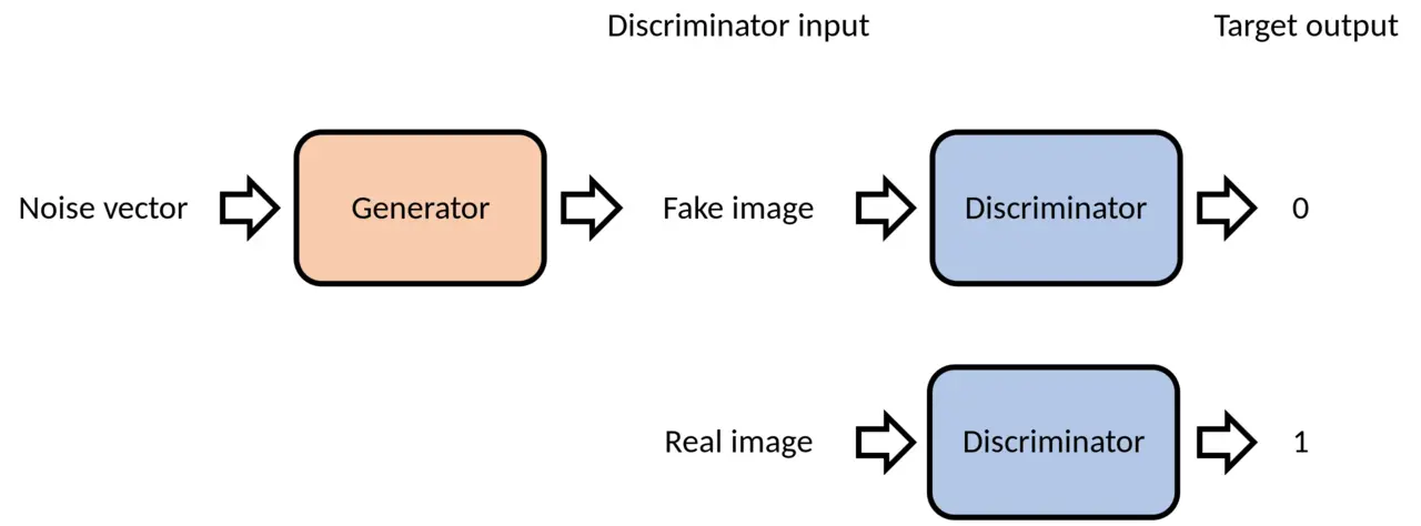
The Generator: The Forger
Role: Create convincing fake data from random noise
The generator network $G$ learns a mapping function: $$z \rightarrow G(z) \approx x_{\text{real}}$$
Where:
- $z$ is a random latent vector (the “noise”)
- $G(z)$ is the generated sample
- The goal is making $G(z)$ indistinguishable from real data
Key insight: The latent space $z$ is continuous, meaning small changes in $z$ produce smooth, meaningful changes in the generated output.
The Discriminator: The Detective
Role: Distinguish between real and generated samples
The discriminator network $D$ outputs a probability: $$D(x) = P(\text{x is real})$$
- $D(x) \approx 1$ for real samples
- $D(x) \approx 0$ for fake samples
It functions as an “authenticity detector” that progressively improves.
The Adversarial Competition
This adversarial dynamic drives the training process. The generator and discriminator have directly opposing objectives:
| Generator Goal | Discriminator Goal |
|---|---|
| Fool the discriminator | Correctly classify all samples |
| Minimize $D(G(z))$ | Maximize $D(x_{\text{real}})$ and minimize $D(G(z))$ |
| “Create convincing fakes” | “Never be fooled” |
This creates a dynamic where both networks continuously improve:
- Generator creates better fakes to fool the discriminator
- Discriminator becomes better at detecting fakes
- The cycle continues until equilibrium

Learning Through Metaphors
Relatable analogies often clarify complex concepts. Here are two metaphors that capture different aspects of how GANs work.
The Art Forger vs. Critic
Generator = Art Forger
Discriminator = Art Critic
A criminal forger tries to create fake masterpieces, while an art critic must identify authentic works. Each interaction teaches both parties:
- The forger learns what makes art look authentic
- The critic develops a keener eye for detecting fakes
- Eventually, the forger becomes so skilled that even experts can’t tell the difference
This captures the adversarial nature and continuous improvement aspect of GANs.
The Counterfeiter vs. Bank Teller
Generator = Counterfeiter
Discriminator = Bank Teller
Day 1: Criminal brings a crayon drawing of a dollar bill. Even a new teller spots this fake.
Day 100: The counterfeiter has learned better techniques. The teller has developed expertise in security features.
Day 1000: The fake money is so convincing that detecting it requires advanced equipment.
This illustrates the progressive improvement and escalating sophistication in both networks.
The Mathematical Foundation
Now let’s examine the mathematical framework that makes GANs work. The core of GAN training is solving a minimax optimization problem.
The Minimax Objective
$$ \min_{G} \max_{D} V(D, G) = \mathbb{E}_{x \sim p_{\text{data}}(x)}[\log D(x)] + \mathbb{E}_{z \sim p_z(z)}[\log(1 - D(G(z)))] $$
Breaking this down:
- $\mathbb{E}_{x \sim p_{\text{data}}(x)}[\log D(x)]$: The expected log-probability for real data.
- Discriminator’s Goal: Maximize this term to correctly classify real samples.
- $\mathbb{E}_{z \sim p_z(z)}[\log(1 - D(G(z)))]$: The expected log-probability for fake data being correctly identified as fake.
- Discriminator’s Goal: Maximize this term.
- Generator’s Goal: Minimize this term to fool the discriminator.
Why “Minimax”?
- Discriminator ($D$): Tries to maximize the objective → Better at distinguishing real from fake.
- Generator ($G$): Tries to minimize the objective → Better at fooling the discriminator.
A Practical Challenge: Vanishing Gradients
The minimax objective presents a practical problem early in training. When the generator is poor, the discriminator can easily distinguish real from fake samples with high confidence ($D(G(z)) \approx 0$). This causes $\log(1 - D(G(z)))$ to saturate and results in vanishing gradients for the generator, which effectively stalls learning.
The Solution: Practitioners typically train the generator to maximize $\log(D(G(z)))$ to provide stronger gradients early in training. This non-saturating heuristic prevents the learning process from stalling.
The Training Process
The beauty of GANs lies in their alternating optimization:
- Fix $G$, train $D$: Make the discriminator optimal for the current generator
- Fix $D$, train $G$: Improve the generator against the current discriminator
- Repeat: Continue until reaching Nash equilibrium
Theoretical Goal: Nash Equilibrium
At convergence, the discriminator outputs $D(x) = 0.5$ for all samples, meaning it can’t distinguish between real and fake data. This indicates that $p_{\text{generator}} = p_{\text{data}}$. Our generator has learned the true data distribution.
The Evolution of Objective Functions
The objective function is the mathematical heart of any GAN. It defines how we measure the “distance” between our generated distribution and the real data distribution. This choice profoundly impacts:
- Training stability: Some objectives lead to more stable convergence
- Sample quality: Different losses emphasize different aspects of realism
- Mode collapse: The tendency to generate limited variety
- Computational efficiency: Some objectives are faster to compute
The original GAN uses Jensen-Shannon Divergence (JSD), but researchers have discovered many alternatives that address specific limitations. Let’s explore this evolution.
The Original GAN: Jensen-Shannon Divergence
The foundational GAN minimizes the Jensen-Shannon Divergence:
$$ \text{JSD}(P, Q) = \frac{1}{2} \text{KL}(P | M) + \frac{1}{2} \text{KL}(Q | M) $$
Where $M = \frac{1}{2}(P + Q)$ is the average distribution, and $\text{KL}$ is the Kullback-Leibler Divergence.
Strengths: Solid theoretical foundation, introduced adversarial training
Limitations: Can suffer from vanishing gradients and mode collapse
Wasserstein GAN (WGAN): A Mathematical Revolution
The Wasserstein GAN revolutionized GAN training by replacing Jensen-Shannon divergence with the Earth-Mover (Wasserstein) distance.
Understanding Earth-Mover Distance
The Wasserstein distance, also known as Earth-Mover distance, has an intuitive interpretation:
Imagine two probability distributions as piles of dirt. The Earth-Mover distance measures the minimum cost to transform one pile into the other, where cost = mass x distance moved.
Mathematically:
$$ W_p(\mu, \nu) = \left( \inf_{\gamma \in \Gamma(\mu, \nu)} \int_{M xM} d(x, y)^p , d\gamma(x, y) \right)^{1/p} $$
Why Earth-Mover Distance Matters
| Jensen-Shannon Divergence | Earth-Mover Distance |
|---|---|
| Can be discontinuous | Always continuous |
| May have vanishing gradients | Meaningful gradients everywhere |
| Limited convergence guarantees | Broader convergence properties |
WGAN Implementation
Since we can’t compute Wasserstein distance directly, WGAN uses the Kantorovich-Rubinstein duality:
- Train a critic function $f$ to approximate the Wasserstein distance
- Constrain the critic to be 1-Lipschitz (using weight clipping)
- Optimize the generator to minimize this distance

Key WGAN Benefits
Meaningful loss function: Loss correlates with sample quality
Improved stability: Less prone to mode collapse
Theoretical guarantees: Solid mathematical foundation
Better convergence: Works even when distributions don’t overlap
Improved WGAN: Solving the Weight Clipping Problem
Improved WGAN (WGAN-GP) addresses a critical flaw in the original WGAN: weight clipping.
The Problem with Weight Clipping
Original WGAN clips weights to maintain the 1-Lipschitz constraint:
# Problematic approach
for param in critic.parameters():
    param.data.clamp_(-0.01, 0.01)
Issues with clipping:
- Forces critic to use extremely simple functions
- Pushes weights toward extreme values ($\pm c$)
- Can lead to poor gradient flow
- Capacity limitations hurt performance
The Gradient Penalty Solution
WGAN-GP introduces a gradient penalty term to constrain the critic:
$$ L = E_{\tilde{x} \sim P_g}[D(\tilde{x})] - E_{x \sim P_r}[D(x)] + \lambda E_{\hat{x}}[(||\nabla_{\hat{x}} D(\hat{x})||_2 - 1)^2] $$
Where $\hat{x}$ are points sampled uniformly along straight lines between real and generated data points.
Advantages:
- No capacity limitations
- Better gradient flow
- More stable training
- Works across different architectures
LSGAN: The Power of Least Squares
Least Squares GAN takes a different approach. It replaces the logarithmic loss with L2 (least squares) loss.
Motivation: Beyond Binary Classification
Traditional GANs use log loss, which focuses primarily on correct classification:
- Real sample correctly classified → minimal penalty
- Fake sample correctly classified → minimal penalty
- Distance from decision boundary ignored
L2 Loss: Distance Matters
LSGAN uses L2 loss, which penalizes proportionally to distance:
$$ \min_D V_{LSGAN}(D) = \frac{1}{2}E_{x \sim p_{data}(x)}[(D(x) - b)^2] + \frac{1}{2}E_{z \sim p_z(z)}[(D(G(z)) - a)^2] $$
$$ \min_G V_{LSGAN}(G) = \frac{1}{2}E_{z \sim p_z(z)}[(D(G(z)) - c)^2] $$
Where typically: $a = 0$ (fake label), $b = c = 1$ (real label)
Benefits of L2 Loss
| Log Loss | L2 Loss |
|---|---|
| Binary focus | Distance-aware |
| Can saturate | Informative gradients |
| Sharp decision boundary | Smooth decision regions |

Key insight: LSGAN minimizes the Pearson χ² divergence, providing smoother optimization landscape than JSD.
Relaxed Wasserstein GAN (RWGAN)
Relaxed WGAN bridges the gap between WGAN and WGAN-GP, proposing a general framework for designing GAN objectives.
Key Innovations
Asymmetric weight clamping: RWGAN introduces an asymmetric approach that provides better balance.
Relaxed Wasserstein divergences: A generalized framework that extends the Wasserstein distance, enabling systematic design of new GAN variants while maintaining theoretical guarantees.
Benefits
- Better convergence properties than standard WGAN
- Framework for designing new loss functions and GAN architectures
- Competitive performance with state-of-the-art methods
Key insight: RWGAN parameterized with KL divergence shows excellent performance while maintaining the theoretical foundations that make Wasserstein GANs attractive.
Statistical Distance Approaches
Several GAN variants focus on minimizing specific statistical distances between distributions.
McGAN: Mean and Covariance Matching
McGAN belongs to the Integral Probability Metric (IPM) family, using statistical moments as the distance measure.
Approach: Match first and second-order statistics:
- Mean matching: Align distribution centers
- Covariance matching: Align distribution shapes
This approach is particularly relevant in scientific simulation, where matching the statistical moments of a generated distribution to the true physical distribution (e.g., molecular conformations) is critical for physical validity.
Limitation: Relies on weight clipping like original WGAN.
GMMN: Maximum Mean Discrepancy
Generative Moment Matching Networks eliminates the discriminator entirely, directly minimizing Maximum Mean Discrepancy (MMD).
MMD Intuition: Compare distributions by their means in a high-dimensional feature space:
$$ \text{MMD}^2(X, Y) = ||E[\phi(x)] - E[\phi(y)]||^2 $$
Benefits:
- Simple, discriminator-free training
- Theoretical guarantees
- Can incorporate autoencoders for better MMD estimation
Drawbacks:
- Computationally expensive
- Often weaker empirical results
MMD GAN: Learning Better Kernels
MMD GAN improves GMMN by learning optimal kernels adversarially to improve upon fixed Gaussian kernels.
Innovation: Combine GAN adversarial training with MMD objective for the best of both worlds.
Different Distance Metrics
Cramer GAN: Addressing Sample Bias
Cramer GAN identifies a critical issue with WGAN: biased sample gradients.
The Problem: WGAN’s Wasserstein distance lacks three important properties:
- Sum invariance (satisfied)
- Scale sensitivity (satisfied)
- Unbiased sample gradients (not satisfied)
The Solution: Use the Cramer distance, which satisfies all three properties:
$$ d_C^2(\mu, \nu) = \int ||E_{X \sim \mu}[X - x] - E_{Y \sim \nu}[Y - x]||^2 d\pi(x) $$
Benefit: More reliable gradients lead to better training dynamics.
Fisher GAN: Chi-Square Distance
Fisher GAN uses a data-dependent constraint on the critic’s second-order moments (variance).
Key Innovation: The constraint naturally bounds the critic without manual techniques:
- No weight clipping needed
- No gradient penalties required
- Constraint emerges from the objective itself
Distance: Approximates the Chi-square distance as critic capacity increases:
$$ \chi^2(P, Q) = \int \frac{(P(x) - Q(x))^2}{Q(x)} dx $$
The Fisher GAN essentially measures the Mahalanobis distance, which accounts for correlated variables relative to the distribution’s centroid. This ensures the generator and critic remain bounded, and as the critic’s capacity increases, it estimates the Chi-square distance.
Benefits:
- Efficient computation
- Training stability
- Unconstrained critic capacity
Beyond Traditional GANs: Alternative Approaches
The following variants explore fundamentally different architectures and training paradigms.
EBGAN: Energy-Based Discrimination
Energy-Based GAN replaces the discriminator with an autoencoder.
Key insight: Use reconstruction error as the discrimination signal:
- Good data → Low reconstruction error
- Poor data → High reconstruction error
Architecture:
- Train autoencoder on real data
- Generator creates samples
- Poor generated samples have high reconstruction loss
- This loss drives generator improvement
Benefits:
- Fast and stable training
- Robust to hyperparameter changes
- No need to balance discriminator/generator
BEGAN: Boundary Equilibrium
BEGAN combines EBGAN’s autoencoder approach with WGAN-style loss functions.
Innovation: Dynamic equilibrium parameter $k_t$ that balances:
- Real data reconstruction quality
- Generated data reconstruction quality
Equilibrium equation:
$$ L_D = L(x) - k_t L(G(z)) $$
$$ k_{t+1} = k_t + \lambda(\gamma L(x) - L(G(z))) $$
MAGAN: Adaptive Margins
MAGAN improves EBGAN by making the margin in the hinge loss adaptive over time.
Concept: Start with a large margin, gradually reduce it as training progresses:
- Early training: Focus on major differences
- Later training: Fine-tune subtle details
Result: Better sample quality and training stability.
Summary: The Evolution of GAN Objectives
The evolution of GAN objective functions reflects the field’s progression toward more stable and theoretically grounded training procedures. Each variant addresses specific limitations in earlier approaches.
Complete Reference Table
| GAN Variant | Key Innovation | Main Benefit | Limitation |
|---|---|---|---|
| Original GAN | Jensen-Shannon divergence | Foundation of adversarial training | Vanishing gradients, mode collapse |
| WGAN | Earth-Mover distance | Meaningful loss, better stability | Weight clipping issues |
| WGAN-GP | Gradient penalty | Solves weight clipping problems | Additional hyperparameter tuning |
| LSGAN | Least squares loss | Better gradients, less saturation | May converge to non-optimal points |
| RWGAN | Relaxed Wasserstein framework | General framework for new designs | Complex theoretical setup |
| McGAN | Mean/covariance matching | Simple statistical alignment | Limited by weight clipping |
| GMMN | Maximum mean discrepancy | No discriminator needed | Computationally expensive |
| MMD GAN | Adversarial kernels for MMD | Improved GMMN performance | Still computationally heavy |
| Cramer GAN | Cramer distance | Unbiased sample gradients | Complex implementation |
| Fisher GAN | Chi-square distance | Self-constraining critic | Limited empirical validation |
| EBGAN | Autoencoder discriminator | Fast, stable training | Requires careful regularization |
| BEGAN | Boundary equilibrium | Dynamic training balance | Additional equilibrium parameter |
| MAGAN | Adaptive margin | Progressive refinement | Margin scheduling complexity |
Practical Recommendations
For practitioners, the choice depends on specific requirements and engineering tradeoffs:
- WGAN-GP: Best balance of stability and performance for most applications. However, tuning the gradient penalty $\lambda$ can be sensitive in practice.
- LSGAN: Simpler implementation with good empirical results.
- EBGAN: Fast experimentation and prototyping.
- Original GAN: Educational purposes and understanding fundamentals.
Real-World Impact: In my work building terabyte-scale VLMs and training models on chaotic physical systems, understanding these foundational dynamics is critical. While we often use diffusion models or autoregressive transformers today, the adversarial training paradigms pioneered by GANs still inform how we stabilize distributed training and design robust loss functions. The choice of objective function fundamentally dictates generation quality, training stability, and computational constraints.
Acknowledgments: This post was inspired by the excellent survey “How Generative Adversarial Networks and Their Variants Work: An Overview of GAN”.